1482 Initial Cover.pdf

n Exchange Rate Policy Rule

Eric Parrado

IDB WORKING PAPER SERIES Nº

IDB-WP-1482

December 2023

Department of Research and Chief Economist

Inter-American Development Bank

December 2023

n Exchange Rate Policy Rule

Eric Parrado

Inter-American Development Bank

Cataloging-in-Publication data provided by the

Inter-American Development Bank

Felipe Herrera Library

Parrado, Eric.

n exchange rate policy rule / Eric Parrado.

p. cm. — (IDB Working Paper Series ; 1482)

Includes bibliographical references.

1. Foreign exchange rates-Singapore. 2. Inflation (Finance)-Singapore. 3. Monetary

policy-Singapore. I. Inter-American Development Bank. Department of Research and

Chief Economist. II. Title. III. Series.

IDB-WP-1482

NonCommercial-NoDerivatives (CC-IGO BY-NC-ND 3.0 IGO) license (http://creativecommons.org/licenses/by-nc-nd/3.0/igo/

legalcode) and may be reproduced with attribution to the IDB and for any non-commercial purpose, as provided below. No

derivative work is allowed.

Any dispute related to the use of the works of the IDB that cannot be settled amicably shall be submitted to arbitration pursuant to

the UNCITRAL rules. The use of the IDB's name for any purpose other than for attribution, and the use of IDB's logo shall be

subject to a separate written license agreement between the IDB and the user and is not authorized as part of this CC-IGO license.

Following a peer review process, and with previous written consent by the Inter-American Development Bank (IDB), a revised

version of this work may also be reproduced in any academic journal, including those indexed by the American Economic

Association's EconLit, provided that the IDB is credited and that the author(s) receive no income from the publication. Therefore,

the restriction to receive income from such publication shall only extend to the publication's author(s). With regard to such

restriction, in case of any inconsistency between the Creative Commons IGO 3.0 Attribution-NonCommercial-NoDerivatives license

and these statements, the latter shall prevail.

Note that link provided above includes additional terms and conditions of the license.

The opinions expressed in this publication are those of the authors and do not necessarily reflect the views of the Inter-American

Development Bank, its Board of Directors, or the countries they represent.

http://www.iadb.org

2023

Abstract

This paper introduces a novel monetary policy framework where the exchange

rate becomes the central instrument. Using Singapore as a case study, it

explores the Monetary Authority's adoption of the exchange rate as the

primary tool since 1981, diverging from conventional approaches centered on

interest rates or monetary aggregates. The estimated exchange rate reaction

function aligns well with actual deviations, supporting the hypothesis that

Singapore’s forward-looking policy rule effectively responds to inflation and

output volatility, especially during economic crises. This framework offers a

promising alternative for countries with open economies and challenges in

implementing traditional interest rate instruments.

JEL classifications: E31, E52, E58, F41

Keywords: exchange rate, inflation, monetary policy rules, Singapore

1. Introduction

Increasing globalization and growing international capital flows have presented significant

challenges in implementing effective monetary policy and selecting appropriate policy

instruments. These challenges are particularly pronounced for small, open economies that strive

to control inflation despite constant foreign shocks. Singapore, recognizing these challenges,

adopted a monetary policy framework centered on managing the exchange rate, with the primary

objective of promoting price stability as the foundation for sustainable economic growth.

Consequently, traditional approaches such as the Taylor rule (Taylor, 1993) or the McCallum rule

(McCallum, 1988), which use interest rates or monetary aggregates, respectively, as policy

instruments, are inadequate for characterizing Singapore’s monetary policy.

In this paper, I build upon Parrado (2004) by introducing a novel policy rule that places the

exchange rate at the core of the monetary policy toolkit. Focusing on Singapore as a case study, I

establish and evaluate a new reaction function to explore how changes in the trade-weighted

nominal exchange rate respond to deviations in inflation and output deviations from their

respective targets. The estimated reaction function reveals a forward-looking approach aimed at

achieving stability in both inflation and output. The strong historical alignment indicates that this

novel reaction function could serve as a valuable benchmark for characterizing monetary policy in

Singapore.

Since 1981, the Monetary Authority of Singapore (MAS) has actively managed the

Singapore dollar’s exchange rate against a trade-weighted basket of currencies representing

Singapore’s major trading partners. The composition of this basket is periodically revised to

accommodate changes in trade patterns, although specific details regarding the index and target-

band boundaries remain undisclosed. The MAS guides the exchange rate to appreciate or

depreciate through direct sales or purchases of the U.S. dollar in the foreign exchange market,

primarily influenced by the strength or weakness of expected inflationary pressures. In essence,

the monetary policy pursued by the MAS follows an unconventional inflation targeting regime.

As the MAS states, “The primary objective has been to promote price stability as a sound

basis for sustainable economic growth. The exchange rate represents an ideal intermediate target

of monetary policy in the context of the small and open Singapore economy. It is relatively

Changes in international reserves Granger-cause changes in the exchange rate.

See Parrado (2004) and McCallum (2014) for further details on monetary policy in Singapore.

controllable through direct interventions in the foreign exchange markets and bears a stable and

predictable relationship with the price stability as the final target of policy over the medium-term.”

The paper is organized as follows. Section 2 provides a summary of Singapore’s

monetary/exchange rate policy framework, and its operation during the past four decades. Section

3 specifies and estimates a policy reaction function for Singapore. In addition, it provides

robustness checks to test the stability of the exchange rate policy rule’s coefficients. Section 4

summarizes the results and derives implications for monetary policy.

2. Background of Singapore’s Monetary Framework

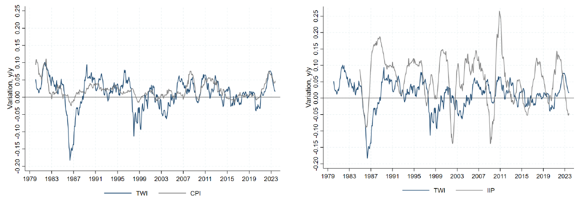
Singapore's exchange-rate-centered monetary policy framework has helped achieve a track record

of low inflation with prolonged economic growth (see Figure 1). Taking advantage of Singapore's

high saving rate, prudent fiscal policy,

4,5

and substantial foreign reserves, monetary policy has

offset inflation pressures by guiding the exchange rate along an appreciating path. At first sight, a

stable rate of inflation has been associated with an appreciating exchange rate. For instance, in the

early 1980s a combination of oil price shocks and high capital flows intensified inflation pressures

in the economy. However, by appreciating the trade-weighted exchange rate index (TWI) by 30

percent during 1981-1985 (averaging about 5 percent per year), inflationary pressures were

contained.

In 1985, Singapore suffered its first recession, caused largely by the deterioration in export

competitiveness, a cyclical downturn in electronics, and the collapse of the construction boom. To

regain competitiveness, a real depreciation was implemented through a reduction in business costs

from a cut in employer pension contributions, and a depreciation of the nominal exchange rate.

The TWI depreciated only by about 16 percent during the 1985-1988 period even though it

depreciated sharply against the Japanese yen and German mark during the period of U.S. dollar

strength following the Plaza Accord. After the economy recovered from the 1985 recession, fear

of renewed inflation prompted the MAS to allow the TWI to appreciate from 1988 through 1997.

Monetary Authority of Singapore (2012).

Continued fiscal surpluses since 1980, except for 1987 and 2001/02, has released the MAS of the need to finance the

government, allowing it to focus on its primarily responsibility of maintaining price stability.

Nadal De Simone (2000) finds that in about 70 percent of the fiscal years between 1967 and 1995, the actual policy

mix in Singapore was a contractionary fiscal policy accompanied by a contractionary monetary policy.

Inflation in Singapore ended around 6 percent annually in the period 1981-82, which contrasts with the OECD

average of nearly 11 percent.

This policy action limited inflationary pressures and precluded an overheated economy during the

first half of the 1990s, when real GDP growth averaged almost 8 percent each year.

With the onset of the Asian crisis, the economy was buffeted by a strengthening of the

Singapore dollar in effective terms, owing to the sharp depreciation of the regional currencies.

Although the Singapore dollar weakened against the U.S. dollar, it strengthened significantly

against the Indonesian rupiah, Thai baht, and Malaysian ringgit. As inflation eased and real GDP

growth stalled, MAS ended its decade-long trend appreciation of the TWI, by easing policy and

guiding the exchange rate to fluctuate within a zero-appreciation exchange rate band. The MAS

also conducted monetary operations to ensure adequate liquidity in the money market, allowing

domestic interest rates to decline.

Figure 1. Evolution of CPI, TWI, and IIP

A. CPI vs TWI B. IIP vs TWI

In early 2000, against the backdrop of a favorable external environment and a strong

rebound in the Singapore economy, monetary policy was tightened by inducing a gradual

appreciation of the Singapore dollar on a trade-weighted basis. MAS announced in January 2001

that it would maintain this policy stance to limit inflation pressures, but economic conditions

subsequently deteriorated by more than expected. Against the backdrop of a weak external

economic environment, a protracted global electronics downturn, and subsiding inflationary

pressures, the MAS eased the policy stance to a neutral setting in July 2001, with a policy band

centered on a zero percent appreciation of the exchange rate.

During the global crisis of 2008, Singapore’s economy experienced a widespread decline,

shrinking by 16.4 percent in the fourth quarter of 2008 on a seasonally adjusted annualized basis

compared to the previous quarter. This downturn was driven by a significant drop in global

demand, leading to a rapid slowdown in sectors linked to trade, including manufacturing,

wholesale trade, and transportation services. Additionally, the financial sector faced severe

challenges due to instability in international financial markets. As a result, the MAS shifted its

policy stance to zero appreciation in April of 2009 and returned to modest appreciation in October

of 2010, when the economy rebounded considerably, and inflation rose to levels above 3 percent.

The outbreak of the COVID-19 pandemic hit the global economy, including Singapore.

Most sectors were affected by the crisis, especially tourism, aviation, retail, and construction. That

year, Singapore’s economy fell 3.9 percent, and inflation was 0 percent, with deflation for 9

consecutive months. MAS opted for a zero-appreciation monetary policy, and the TWI fell nearly

3 percent in 2020.

During 2021 and 2022, Singapore’s economy recovered, largely due to the easing of some

COVID-19 restrictions, robust fiscal stimuli, and monetary policy easing. This recovery also

brought with it demand pressures, which combined with persistent global supply chain disruptions

and the onset of the war in Ukraine, contributed to a substantial rise in inflation. Price increases

peaked in August of 2022, reaching 7.4 percent. In response to these inflationary pressures, the

Monetary Authority of Singapore (MAS) tightened monetary policy by re-centering the mid-point

of the Singapore dollar nominal effective exchange rate policy band and slightly increasing the

rate of appreciation of the policy band.

With this background, the next sections analyze the determinants of inflation as a basis for

specifying a policy reaction function that could reproduce these historical shifts in the policy

stance. The impact of the direct effects of the exchange rate on inflation and its indirect effects

through output changes will shed light on the transmission channels of monetary policy. The

estimated reaction function would be used to gauge how changes in economic fundamentals

influence changes in the monetary policy stance, as reflected in the changes in the TWI.

3. Exchange Rate Policy: A Proposal

3.1 Specification

Here, the conventional empirical policy reaction functions, in which a domestic interest rate or

monetary aggregate is the policy variable, are modified to allow the monetary policy stance to be

characterized by changes in the trade-weighted exchange rate index (TWI) or the Singapore

dollar’s nominal effective exchange rate.

The policy reaction function works as follows: Assume that within each operating period

the MAS has a target for the change in the TWI, , that is based on the state of the economy.

Also assume that the MAS cares about stabilizing inflation and output, while allowing for the

possibility that it adjusts its policy response to anticipated inflation and output. Specifically:

, (1)

where is the long-run equilibrium change in the TWI, is the rate of inflation between

periods t and t+n, is real output (or industrial production) between periods t and t+m, and

and are the targets for inflation and output, respectively. In particular, is defined as the

equilibrium level of output that would arise if wages and prices were perfectly flexible. E is the

expectation operator, and is the information available to the policymaker.

To capture concerns about potentially disruptive shifts in the exchange rate, I assume that

the exchange rate is adjusted only partially to its target level:

. (2)

Here, the parameter captures the degree of exchange rate smoothing. The exogenous

random shock to the exchange rate, , is assumed to be i.i.d.

To define an estimable equation, let

α βπ

=∆−

and . Then equation (1) can

be rewritten as follows:

. (3)

Combining equation (3) with the partial adjustment mechanism (2) and eliminating the

unobserved forecast variables yields the following:

e∆

[ ]

( )

[ ]

( )

* **

t tn t tm t

e e E Ey y

βπ πγ

∆ =∆+ Ω− + Ω−

e∆

Ω

( )

t t tt

e ee

ρ ρυ

−

∆ = − ∆ +∆ +

[ ]

0,1

∈

xyy= −

[ ] [ ]

t tn t tm t

e E Ex

αβ π γ

∆ = + Ω+ Ω

. (4)

The error term is a linear combination of the forecast errors of inflation and output and the

exogenous disturbance .

This new policy rule deviates from the conventional Taylor and McCallum rules, which

typically rely on short-term interest rates or monetary aggregates as monetary policy instruments.

Parrado (2004) proposed a novel approach in which the change in the exchange rate serves as the

key monetary policy instrument in a forward-looking inflation targeting context. This innovative

perspective opened new avenues for research. Subsequently, several other scholars have

incorporated this distinctive exchange rate rule into their own analyses.

Let be a vector of variables (a set of instruments) within the policymaker’s information

set (i.e., ) that are orthogonal to . Possible elements of include any lagged variables

that help forecast inflation and output and any contemporaneous variables that are uncorrelated

with the current exchange rate shock . In particular, the choice of instruments used in this paper

includes 1 to 12 lags of the Consumer Price Index (CPI) inflation, industrial production gap, the

TWI, the World Commodity Index, and the nominal federal funds rate. Contemporaneous CPI

inflation and TWI are also included as instruments.

Thus, since , the following equation can be estimated using the Generalized

Method of Moments (GMM) with an optimal weighting matrix:

. (5)

3.2 Estimation

Equation (5) is estimated over the sample period from 1985:01 to 2023:04 with year-on-year CPI,

year-on-year industrial production, and the year-on-year change in the TWI. The elements of

are lagged values of CPI inflation, output, the TWI, the International Monetary Fund’s World

See Gerlach-Kristen (2006), Gerlach and Gerlach-Kristen (2006), McCallum (2007), Khor et al. (2007), MAS

(2013), Mihov (2013), Santacreu (2015), Benes et al. (2015), Corbacho and Peiris (2018), Heipertz et al. (2022), and

Cavoli et al (2023), among others.

The use of an optimal weighting matrix implies that GMM estimates are robust to heteroskedasticity and

autocorrelation of unknown form.

( ) ( ) ( )

11 1

t tn tm t t

e xe

ρ α ρ βπ ρ γ ρ ε

+ +−

∆=− +− +− +∆ +

u ∈Ω

[ ]

( ) ( ) ( )

1 1 1 |0

t tn tm t t

Ee x eu

ρ α ρ βπ ρ γ ρ

+ +−

∆−− −− −− −∆ =





Commodity Price Index, and the nominal federal funds rate.

The forward-looking horizons are

varied to assess the policy horizon.

Assuming a forward-looking horizon of nine months (n = 9)—at which the standard error

of the regression is the smallest and the

is the largest—the coefficients associated with expected

inflation are positive and significant (see Table 1). They indicate that, in response to a 1 percent

rise in expected inflation, the TWI is appreciated by 1.8 percent, implying a real exchange rate

appreciation of 0.8 percent, ceteris paribus. In other words, the real exchange rate is temporarily

altered to affect aggregate demand, and thus, inflation. The coefficient associated with the

industrial output gap is also positive and significant, suggesting that the monetary authority reacts

by appreciating the exchange rate by 0.48 percent when domestic output is 1 percent above

potential. Finally, the coefficient that captures policy inertia is high (ρ ≅ 0.93), indicating that

monetary policy slowly adjusts the exchange rate to its projected target level.

10,11

Table 1. The MAS Reaction Function

Baseline Case

Alternative Inflation Target

Horizons

α β γ ρ

p-value J-test

Current inflation (n=0)

0.0010

0.784**

0.695***

0.929***

0.930 0.533 58.449

(0.074)

(2.158)

(4.436)

(81.307)

Expected inflation (n=3)

-0.0100

1.356***

0.539***

0.923***

0.931 0.547 58.059

(-1.288)

(4.052)

(3.929)

(85.828)

Expected inflation (n=6)

-0.0120

1.473***

0.523***

0.927***

0.931 0.531 58.505

(-1.372)

(3.529)

(3.459)

(86.544)

Expected inflation (n=9)

-0.019*

1.813***

0.479***

0.927***

0.931 0.508 59.113

(-1.804)

(3.702)

(3.263)

(87.095)

Expected inflation (n=12)

-0.025**

2.078***

0.513***

0.927***

0.930 0.494 59.501

(-2.07)

(3.746)

(3.928)

(87.081)

(1) * p<0.10; ** p<0.05; *** p<0.01.

(2) t statistics are in parentheses.

(3) The set of instruments includes 1 to 12 lags of CPI inflation, the industrial production gap, the TWI, the World Commodity

Index, and the nominal federal funds rate. Contemporaneous CPI inflation and TWI are also included as instruments.

(4) Data range from January 1985 to April of 2023.

Source: Author’s estimates.

Sargan-Hansen J-test is also performed to avoid overidentification.

Additional estimates confirm that a standard Taylor rule is not observationally equivalent.

The estimated coefficients associated with inflation are stable for several specifications and combinations of

different target horizons for the output gap (m=3,6,9,12).

These results are corroborated by two additional exercises that test the hypothesis that

Singapore’s monetary policy reacts mainly to large shocks. Table 2 includes only large

fluctuations (larger than half a standard deviation) in CPI inflation. The results confirm that

monetary policy reacts to large changes in inflation, as the beta coefficient continues to be

significant. Conversely, regressions (not reported here) suggest that monetary policy hardly

responds to small shocks.

Table 2. The MAS Reaction Function

High Inflation Volatility

Alternative Inflation Target

Horizons

α β γ ρ

p-value J-test

Current inflation (n=0)

-0.0050

0.816**

0.646***

0.944***

0.947 0.849 48.805

(0.009)

(0.326)

(0.168)

(0.011)

Expected inflation (n=3)

-0.023***

1.461***

0.356***

0.923***

0.943 0.943 43.719

(0.007)

(0.261)

(0.097)

(0.011)

Expected inflation (n=6)

-0.0170

1.51***

0.503***

0.944***

0.937 0.933 44.461

(0.012)

(0.453)

(0.152)

(0.009)

Expected inflation (n=9)

-0.044**

2.325***

0.452**

0.953***

0.926 0.928 44.809

(0.017)

(0.635)

(0.192)

(0.011)

Expected inflation (n=12)

-0.0140

1.365***

0.705***

0.93***

0.917 0.911 45.853

(0.011)

(0.387)

(0.182)

(0.014)

(1) * p<0.10; ** p<0.05; *** p<0.01.

(2) t statistics are in parentheses.

(3) The set of instruments includes 1 to 12 lags of CPI inflation, the industrial production gap, the TWI, the World Commodity

Index, and the nominal federal funds rate. Contemporaneous CPI inflation and TWI are also included as instruments.

(4) Data range from January 1985 to April of 2023.

Source: Author’s estimates.

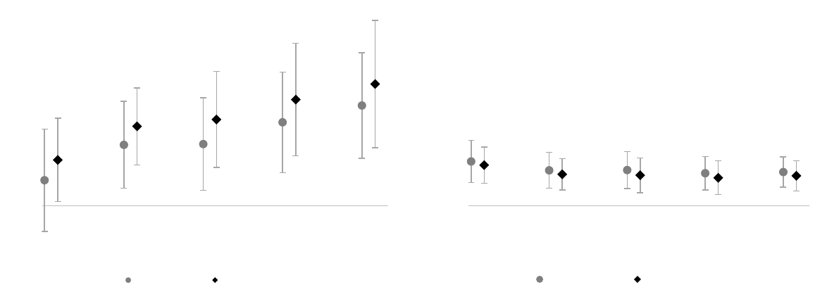
In addition to assessing the MAS’s reaction to significant shocks, I estimate the coefficients

using a sample that excludes the 2008-09 financial crisis and the COVID-19 pandemic. These

estimations are then compared with the coefficients obtained from the analysis of the entire sample.

When the crises are considered, the beta coefficients exhibited higher values, indicating a more

substantial policy response when the economy faces a recession (see Figure 2). At the same time,

the gamma coefficients (associated with the output gap) are slightly lower. These findings shed

light on the MAS’s dynamic policy approach during economic downturns.

Figure 2. Estimated Coefficients of Inflation Gap (Beta) and Output Gap (Gamma)

Different samples (whole sample vs w/o crises)

(1) The set of instruments includes 1 to 12 lags of CPI inflation, the industrial production gap, the TWI, the World

Commodity Index, and the nominal federal funds rate. Contemporaneous CPI inflation and TWI are also included as

instruments.

(2) The data range between 1985:01 – 2007:12 and 2010:01 - 2019:12 when the 2008-09 financial crisis and the

COVID-19 crisis are excluded.

Source: Author’s calculations.

3.3 Robustness

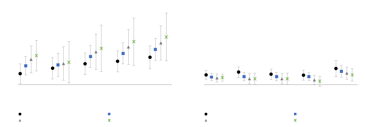
3.3.1 Targets Horizons

The decision to select a fixed target horizon of zero (m=0) for the output gap in the analysis was

primarily driven by simplicity. Given that the original exercise already incorporates multiple target

horizons for the inflation gap, including various combinations with the output gap could introduce

confusion. However, it is crucial to examine the stability of the parameter associated with the

inflation gap.

Figure 3 illustrates the stability of the estimated coefficient associated with inflation across

various specifications. Notably, the statistical analysis reveals that most betas and gammas exhibit

strong levels of significance. However, there are a few exceptions: notably, the gamma value does

not achieve significance when the inflation horizon (n) is set at 12 and the output horizon (m) is

either 3 or 9.

-0.5

0.0

0.5

1.0

1.5

2.0

2.5

3.0

0 3 6 9 12

Coefficient

Inflation horizon (n)

A. Beta

Without crises Whole sample

-0.5

0.0

0.5

1.0

1.5

2.0

2.5

3.0

0 3 6 9 12

Coefficient

Inflation horizon (n)

B. Gamma

Without crises Whole sample

Figure 3. Estimated Coefficients Inflation Gap (Beta) and Output Gap (Gamma)

Different output horizons

(1) The set of instruments includes 1 to 12 lags of CPI inflation, the industrial production gap, the nominal effective

exchange rate, the world commodity price index and the nominal federal funds rate. Contemporaneous CPI inflation

and TWI are also included as instruments.

Source: Author’s estimates.

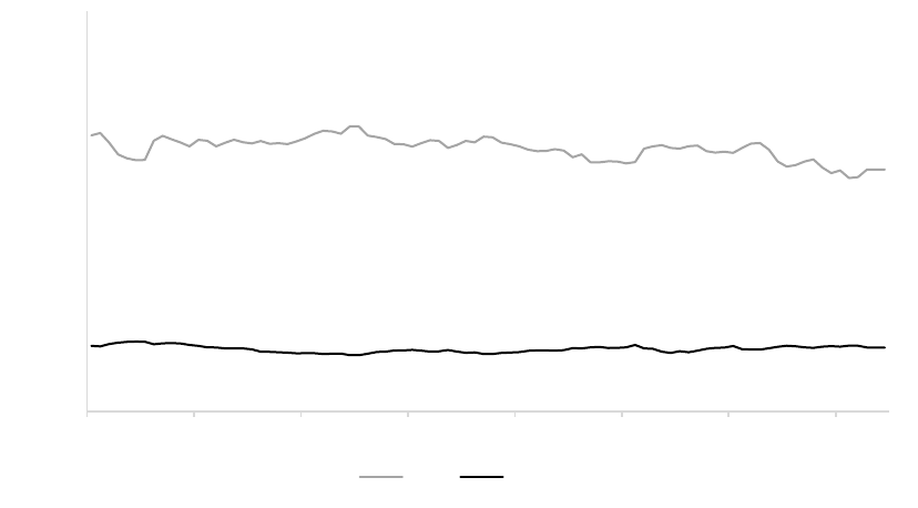
3.3.2 Samples

Overall, the estimated parameters exhibit stability when employing various samples, including the

rho estimates. This observation is further supported by the findings presented in Figure 4. In this

analysis, the sample range is initially restricted to 2014:12, and each subsequent monthly

observation is cumulatively added. Importantly, the results demonstrate consistent stability across

the entire timeline, and they remain statistically significant.

-1

0 3 6 9 12

Coefficient

Output horizon (m)

A. Beta

β (Inflation horizon = 0) β (Inflation horizon = 3)

β (Inflation horizon = 9) β (Inflation horizon = 12)

-1

0 3 6 9 12

Coefficient

Output horizon (m)

B. Gamma

β (Inflation horizon = 0) β (Inflation horizon = 3)

β (Inflation horizon = 9) β (Inflation horizon = 12)

Figure 4. Beta and Gamma with Different Time Horizons

Expected inflation = 9

(1) All coefficients are statistically significant at the 95 percent level.

(2) The set of instruments includes 1 to 12 lags of CPI inflation, the industrial production gap, the TWI, the World

Commodity Index, and the nominal federal funds rate. Contemporaneous CPI inflation and TWI are also included as

instruments.

Source: Author’s estimates.

3.3.2 Selection of Instruments and Lags

The set of instruments in this study encompasses all the variables within the MAS’s information

set when changes in the exchange rate—the policy variable—occur. A similar approach is

discussed by Favero (2000), who notes that a vector should incorporate all the variables available

to the central bank when making decisions on interest rates. Furthermore, to evaluate whether the

simple specification of the monetary policy rule overlooks significant variables that are part of the

central bank’s rule, the standard statistical analysis employs the J-test to assess the validity of

overidentifying restrictions.

Regarding the inclusion of lags, Clarida, Galí, and Gertler (2000) argue that the instruments

used should be based on the information set available when determining the interest rate. They

incorporate four lags of inflation, the output gap, the federal funds rate, the short-long spread, and

commodity price inflation in estimating the Federal Reserve’s policy reaction function.

Similarly, Caputo and Herrera (2017) use lagged values of country-specific output,

inflation deviations, the policy rate, exchange rate changes, and contemporaneous and lagged

0.0

0.5

1.0

1.5

2.0

2.5

3.0

2015 2016 2017 2018 2019 2020 2021 2022

Coefficient

Sample's upper range

Beta Gamma

values of common variables such as the fed funds rate and the percentage change in oil prices for

each country. Additionally, contemporaneous inflation is included as an instrument.

4. Conclusion

The estimation results from the reaction function analysis provide compelling evidence that

controlling inflation has been the primary focus of monetary policy in Singapore. This supports

the hypothesis that the monetary policy framework in Singapore can be characterized by a forward-

looking policy rule that aims to stabilize expected inflation and maintain output at its potential

level. Notably, the estimated reaction function implicitly includes an inflation targeting

component, as argued by Clarida, Galí, and Gertler (1998, 1999), highlighting its significance in

ensuring effective monetary policy making.

Furthermore, the coefficients associated with CPI inflation and output reveal that monetary

policy in Singapore assigns considerable importance to maintaining low and stable inflation.

Importantly, the estimations demonstrate stability across samples, suggesting the findings are

robust. When crises such as the 2008-9 financial crisis and the COVID-19 pandemic are

considered, the coefficient associated with expected inflation is larger. This implies that the policy

response is more pronounced during economic downturns, underlining the adaptive nature of

monetary policy in addressing recessions.

Given the strong historical fit of the estimated reaction function, this approach presents a

promising alternative for countries with high openness to capital markets that face challenges in

managing monetary policy effectively using traditional instruments such as interest rates or

monetary aggregates. In fact, recent research building upon this framework suggests that when a

small and open economy has a trade openness level above 40 percent of GDP, a monetary policy

framework centered on an exchange rate instrument is more efficient in stabilizing prices than the

traditional interest rate approach (Heresi and Parrado, 2023).

References

Benes, J., A. Berg, R. Portillo, and D. Vavra. 2015. “Modeling Sterilized Interventions and

Balance Sheet Effects of Monetary Policy in a New-Keynesian Framework.” Open

Economies Review 26: 81-108.

Caputo, R., and L.O. Herrera. 2017. “Following the Leader? The Relevance of the Fed Funds Rate

for Inflation Targeting Countries.” Journal of International Money and Finance 71: 25-52.

Cavoli, T., S. Gopalan, and R.S. Rajan. 2023, “Is Exchange Rate Centred Monetary Policy

Asymmetric? Empirical Evidence from Singapore.” Applied Economics 55(21): 2438-

2454.

Clarida, R., J. Galí, and M. Gertler. 1998. “Monetary Policy Rules in Practice: Some International

Evidence.” European Economic Review 42(6): 1033-1067.

Clarida, R., J. Galí, and M. Gertler. 1999. “The Science of Monetary Policy: A New Keynesian

Perspective.” Journal of Economic Literature 37(4): 1661–1707.

Clarida, R., J. Galí, and M. Gertler. 2000. “Monetary Policy Rules and Macroeconomic Stability:

Evidence and Some Theory.” Quarterly Journal of Economics 115(1): 147-180.

Corbacho, A., and S.J. Peiris. 2018. “Monetary and Exchange Rate Policy Responses.” In: A.

Corbacho and S.J. Peiris, editors. The Asean Way: Sustaining Growth and Stability.

Washington, DC, United States: International Monetary Fund.

Favero, C. 2000. “New Econometric Techniques and Macroeconomics.” In: R. Backhouse, editor.

Macroeconomics and the Real World. Oxford, United Kingdom: Oxford University Press.

Gerlach-Kristen, P. 2006. “Internal and External Shocks in Hong Kong: Empirical Evidence and

Policy Options.” Economic Modelling 23: 56-75.

Gerlach, S., and P. Gerlach-Kristen. 2006. “Monetary Policy Regimes and Macroeconomic

Outcomes: Hong Kong and Singapore.” BIS Working Paper 204. Basel, Switzerland: Bank

for International Settlements.

Hansen, L. 1982. “Large Sample Properties of Generalized Method of Moments Estimators.”

Econometrica 50(4): 1029–54.

Heipertz, J., I. Mihov, and A.M. Santacreu. 2022. “Managing Macroeconomic Fluctuations with

Flexible Exchange Rate Targeting.” Journal of Economic Dynamics and Control 135:

104311.

Heresi, R., and E. Parrado. 2023. “Trade Openness and the Optimal Degree of Exchange Rate

Management.” Washington, DC, United States: Inter-American Development Bank.

Unpublished manuscript

Khor, H.E., J. Lee, E. Robinson, and S. Supaat. 2007. “Managed Float Exchange Rate System:

The Singapore Experience.” Singapore Economic Review 52(1): 7-25.

McCallum, B. 1988. “Robustness Properties of a Rule for Monetary Policy.” Carnegie-Rochester

Conference on Public Policy 29: 173-204.

McCallum, B. 2007. “Monetary Policy in East Asia: The Case of Singapore.” IMES Discussion

Paper 2007-E-10. Tokyo, Japan: Bank of Japan, Institute for Monetary and Economic

Studies.

McCallum, B. 2014. “Monetary Policy in a Very Open Economy: Some Major Analytical Issues.”

Pacific Economic Review 19: 27-60.

Mihov, I. 2013. “The Exchange Rate as an Instrument of Monetary Policy.” MAS Macroeconomic

Review 12(1): 74–82.

MAS. 2012. “Singapore’s Exchange Rate-Based Monetary Policy.”

MAS. 2013. “Macroeconomic Developments.” MAS Macroeconomic Review 12(1): 2-14.

Nadal de Simone, F. 2000. “Monetary and Fiscal Policy Interaction in a Small Open Economy:

The Case of Singapore.” Asian Economic Journal 14(2): 211-31.

Parrado, E. 2004. “Singapore’s Unique Monetary Policy: How Does it Work?” IMF Working

Paper 04/10. Washington, DC, United States: International Monetary Fund.

Santacreu, A.M. 2015. “Monetary Policy in Small Open Economies: The Role of Exchange Rate

Rules.” Federal Reserve Bank of St. Louis Review 97(3): 217-32.

Taylor, J. 1993. “Discretion versus Policy Rules in Practice.” Carnegie-Rochester Conference

Series on Public Policy 39: 195-214.