Singapore: Selected Issues; IMF Country Report 08/281; July 1, 2008

IMF Country Report No. 08/281

Singapore: Selected Issues

This Selected Issues paper for Singapore was prepared by a staff team of the International Monetary

Fund as background documentation for the periodic consultation with the member country. It is based

on the information available at the time it was completed on July 1, 2008. The views expressed in this

document are those of the staff team and do not necessarily reflect the views of the government of

Singapore or the Executive Board of the IMF.

The policy of publication of staff reports and other documents by the IMF allows for the deletion of

market-sensitive information.

Copies of this report are available to the public from

International Monetary Fund ● Publication Services

700 19th Street, N.W. ● Washington, D.C. 20431

Telephone: (202) 623-7430 ● Telefax: (202) 623-7201

E-mail: publicati[email protected]g

● Internet: http://www.imf.org

Price: $18.00 a copy

International Monetary Fund

Washington, D.C.

INTERNATIONAL MONETARY FUND

SINGAPORE

Selected Issues

Prepared by Leif Eskesen and Roberto Guimaraes-Filho (both APD),

Elena Loukoianova and Miguel Segoviano (both MCM)

Approved by the Asia and Pacific Department

July 1, 2008

Contents Page

Executive Summary ........................................................................................................... 2

I. Assessing the Stability of Singapore’s Banking System in a Regional Context ......... 3

A. Introduction............................................................................................................. 3

B. Analytical Framework............................................................................................. 4

C. Main Findings ......................................................................................................... 6

D. Concluding Remarks............................................................................................. 10

References.................................................................................................................. 12

II. The Effects of Monetary Policy in Singapore............................................................ 13

A. Introduction........................................................................................................... 13

B. Inflation in Singapore: Some Stylized Facts......................................................... 14

C. Data and Empirical Model .................................................................................... 15

D. Main Findings ....................................................................................................... 16

E. Concluding Remarks ............................................................................................. 18

Annex II.1. Estimation Details................................................................................... 20

References.................................................................................................................. 22

III. Effectiveness of Fiscal Policy in Singapore............................................................... 23

A. Introduction........................................................................................................... 23

B. Cross-country Evidence on the Effectiveness of Fiscal policy............................. 24

C. Effectiveness of Fiscal Policy in Singapore.......................................................... 26

D. Concluding Remarks............................................................................................. 28

Annex III.1. Technical Description of the Fiscal SVAR Framework........................ 30

References.................................................................................................................. 33

EXECUTIVE SUMMARY

The ongoing turbulence in the world’s economy and financial markets provides an

opportunity to assess Singapore’s exposure to international spillovers and possible policy

responses. This Selected Issues paper accompanies the Staff Report for the 2008 Article IV

consultation with Singapore and offers analytical underpinnings for the staff’s views on

international financial linkages and the effectiveness of monetary and fiscal policy. It

consists of three chapters:

Chapter I—Assessing the Stability of Singapore’s Banking System in a Regional Context—

proposes a novel methodology for gauging domestic financial stability. The methodology

gives preliminary estimates of measures of default interdependence between Singaporean and

selected regional banks operating domestically. The analysis supports the staff’s view that

Singaporean banks have been resilient to the global financial turmoil, thus far.

Chapter II—The Effects of Monetary Policy in Singapore—analyzes the effects of monetary

policy using structural vector autoregressions. Estimates show that the Monetary Authority of

Singapore’s exchange rate-centered framework is well suited to shape monetary decision

making, given the large impact that changes in the nominal exchange rate have on activity

and prices. The results are consistent with the staff’s recommendation that a faster rate of

appreciation of the Singapore dollar would help contain inflation risks, going forward.

Chapter III—Effectiveness of Fiscal Policy in Singapore—assesses the impact of fiscal

measures on macroeconomic activity. Econometric results confirm a role for fiscal policy as

a counter-cyclical tool and support the staff‘s view that a carefully designed fiscal stimulus

should play a part in re-orienting the policy mix to facilitate external adjustment.

I. ASSESSING THE STABILITY OF SINGAPORE’S BANKING SYSTEM IN A REGIONAL

CONTEXT

This chapter proposes a methodology for assessing the stability of the banking system in

Singapore in a regional Asian context. The methodology allows for a quantification of the

evolution of default interdependence of Singaporean and selected regional banks. The main

results of the analysis indicate that the largest Singaporean banks have remained resilient to

the global financial turmoil and have generally been less affected than regional banks

operating in Singapore.

A. Introduction

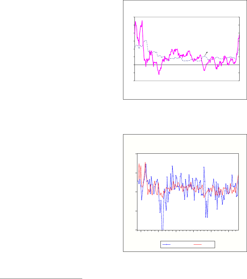
1. The direct impact of the global credit turmoil on Singaporean banks has been

limited so far. Credit default swap (CDS) spreads for Singaporean and Asian banks

increased significantly since the second half of 2007 on the back of the global credit turmoil

and have remained elevated even after a decline since March 2008. However, the reported

subprime related exposures and estimated losses of Singaporean banks are lower than

elsewhere in Asia, and in the United States and Europe. Moreover, Singaporean banks have

made prudent provisions against losses on exposures to the U.S. subprime related assets.

Banks: Credit Default Swap Spreads

100

150

200

250

300

Jul-07 Sep-07 Nov-07 Jan-08 Apr-08

100

150

200

250

300

Singapore

Japan

Korea

Australia

Stock Market Indices

(2000M1=100)

-50

100

150

200

250

300

350

400

450

Jan-00 Jan-01 Jan-02 Jan-03 Jan-04 Jan-05 Jan-06 Jan-07 Jan-08

-50

100

150

200

250

300

350

400

450

Singapore

Hong Kong SAR

China (Shanghai)

Korea

Malaysia

Thailand

2. This chapter assesses the stability of the banking sector in Singapore using a

novel methodology. The methodology is still work in progress and the results should be

interpreted with care. The central insight is to derive the probabilities of default (PoDs) of a

sample of Singaporean and regional banks and estimate the joint probability of default

(JPoD) and other conditional measures of banking sector stability. The chapter proceeds as

follows: Section B summarizes the analytical framework, Section C presents the main

finding, and section D concludes.

Prepared by Elena Loukoianova and Miguel Segoviano (both MCM).

B. Analytical Framework

3. The analysis provides novel measures of banking stability and contributes to the

modeling of default risk. It extracts market information to assess potential contagion effects

and the resilience among Singaporean and selected regional banks operating in Singapore.

The exercise provides a new methodology and complements the study presented in the

special feature in the 2007 Monetary Authority of Singapore’s Financial Stability Review.

4. The central idea behind the methodology is to treat the banking system as a

“portfolio of banks.” The estimates of banking system stability capture risks of the

individual banks and interdependencies of the banks in the portfolio.

The model is applied to

a portfolio of Singaporean banks only and one of Singaporean and regional banks.

5. The analytical framework uses two variables to estimate different measures of

banking stability: daily equity prices and daily CDS spreads.

Equity prices are used to

calibrate the initial conditions for model simulations.

Based on the PoDs for individual

banks extracted from CDS spreads, the framework then computes a multivariate density

function (PMD) to capture the implied distribution of asset values of the banks included in

the portfolio.

The PMD embeds the default dependence among the banks in the portfolio

and allows for the estimation of the JPoD of the bank portfolio under consideration.

The methodology proposed here can be applied to alternative inputs for calculating PoDs of individual banks

and JPoDs of different bank groups.

The special feature used panel data econometric estimates and analyzed data for the period from January 2002

to December 2006—prior to the onset of the credit turmoil in mid-2007. This analysis found that the East Asian

banking systems became more resilient after the Asian financial crisis, the default risk of banks declined, and

contagion among banks also declined. The MAS attributed lower default risk to income diversification.

Goodhart and Segoviano, 2008. Box 1.5 in the April 2008 GFSR presents an application of this methodology

for a group of large financial institutions.

A number of multinational banks have branches in Singapore and thus have a bearing on domestic financial

stability. Lack of branch-level data precludes, however, a quantitative analysis of the issue

The data for both variables are from Bloomberg.

See Segoviano (2008) for details on calculation of PoDs.

Segoviano, 2008.

Under the probability integral transformation (PIT) criterion, the PMD produced by nonparametric techniques

is an improvement over standard parametric PMDs used for modeling portfolio credit risks (See Diebold et al.

(1999) for details).

The methodology proposes a novel nonparametric copula approach―which assumes neither a particular

distribution nor parameters, thus making possible a better fit to the data. The structure of linear and nonlinear

(continued)

6. The JPoD represents the unconditional probability of default of all the banks in

the sample, i.e. the tail risk of the system. The JPoD accounts for the nonlinear

dependencies among banks in this portfolio of banks.

In periods of financial distress, the

JPoD of the banking system may experience larger fluctuations compared with those of the

PoDs of individual banks because of stronger interdependencies during times of stress.

7. The JPoD provides the base for calculating conditional measures of banking

stability:

• The Banking Stability Index (BSI), which shows the expected number of bank

defaults, conditional on at least one bank defaulting.

• The Default Dependence Matrix (DDM), which is a matrix of pairwise conditional

probabilities of default, indicating the probability of default of a bank in the row,

given that a bank in the column defaults;

• The Conditional Systemic Relevance Factor (SRF), which reflects the probability of

default of all the banks in the system conditional on the default of a specific bank; and

• The Conditional Resilience Factor (RF), which indicates the opposite of the SRF,

namely the probability that a bank defaults conditional on the default of all the other

banks.

8. The methodology is subject to some data limitations when applied to emerging

market countries. First, inputs (equity prices and CDS spreads) used may not be the best

proxy for estimating banks’ probabilities of default, especially in times of global market

turmoil.

Second, limited data availability on CDS spreads constrains the choice of banks,

dependencies among banks in a system can be represented by copula functions. This approach infers copulas

from the joint movements of PoDs of individual banks, thus avoiding the difficulties involved in explicitly

choosing and calibrating individual measurements of banks’ defaults. This is the main contrast between and

traditional copula modeling approaches, as explicit calibration in most cases is difficult because of data

constraints.

Accounting for nonlinear dependencies changing over time is a relevant technical improvement over most

risk models, which typically account only for dependencies that are assumed constant over the cycle.

The BSI is conditional of a default of any bank in the system, but not a specific bank. Moreover, such a

default might never materialize.

In the current episode, the risk landscape and consequently hedging strategies have shifted significantly since

June 2007. The discrepancy between CDS spreads and bond prices, coupled with the increasing illiquidity of

the credit markets (especially for CDS spreads of local banks), has clouded the information embedded in the

CDS spreads.

which may result in a sample that is not fully representative of the banking sector under

consideration.

C. Main Findings

9. An assessment of banking sector vulnerabilities involves a careful evaluation of a

broad spectrum of indicators, in changes and levels. Changes bespeak the impact from

global financial reverberations, while levels provide evidence of resilience. In the case of

Singapore, changes in the indicators confirm international spillovers, but the absolute levels

of the measures suggest that overall resilience of the Singaporean banking system remains

high. As regards linkages with regional banks, evidence is more ambiguous. In particular:

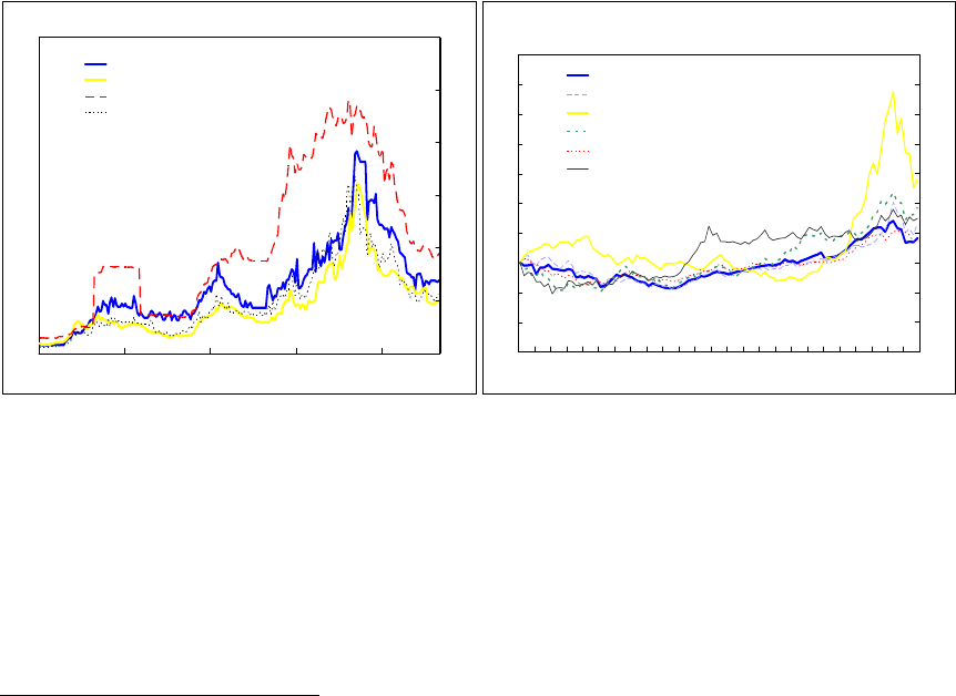
• The PoDs and the JPoDs of both bank groups analyzed increased as the global credit

crisis unfolded. Between the end of July 2007 and the end of March 2008, the average

PoD of the institutions in the “Singaporean bank” portfolio increased by about

7 times, while their JPoD increased by a larger factor.

The average PoD of the group

of “Singaporean and regional” banks increased by 3½ times, while its JPoD rose by

even more (Figures I.1 and I.2). The significant difference between the magnitude of

increases in the average PoDs and the JPoDs reveals large increases in default

interdependence among the banks during this period of financial distress. The JPoD

of the Singaporean-regional bank portfolio is smaller than that of the Singaporean

bank portfolio, which could reflect diversification gains and/or a nonrepresentative

sample. Because of the data limitations mentioned above, this evidence needs to be

interpreted carefully.

Figure I.1. Marginal Probabilities of Default

Singaporean banks Singaporean-Regional banks

0.000

0.005

0.010

0.015

0.020

0.025

0.030

0.035

0.040

12/1/2006 3/1/2007 6/1/2007 9/1/2007 12/1/2007 3/1/2008

Sing.bank 1

Sing.bank 2

Sing.bank 3

0.000

0.005

0.010

0.015

0.020

0.025

0.030

0.035

0.040

0.045

0.050

12/1/2006 3/1/2007 6/1/2007 9/1/2007 12/1/2007 3/1/2008

Sing.bank 2

Sing.bank 3

Sing.bank 1

Reg.bank 1

Reg.bank 2

Reg.bank 3

The average PoD is defined here as a simple average of the PoDs of individual banks in a group.

Figure I.2. Joint Probability of Default and Average Marginal Probability

Singaporean banks Singaporean-Regional banks

0.001

0.002

0.003

0.004

0.005

0.006

0.007

0.008

0.009

12/01/06 02/23/07 05/18/07 08/10/07 11/02/07 01/25/08

0.000

0.005

0.010

0.015

0.020

0.025

0.030

0.035

JPoD (left axis)

Average PD (right axis)

0.000

0.005

0.010

0.015

0.020

0.025

0.030

0.035

12/01/06 02/23/07 05/18/07 08/10/07 11/02/07 01/25/08

0.001

0.002

0.003

0.004

0.005

0.006

Average PD (left axis)

JPoD (right axis)

• The BSI shows signs of an adverse impact from the global turmoil on Singapore’s

banking sector, but largely through regional banks (Figure I.3). For the group of

Singaporean banks, the BSI increased by only 0.5 reaching 1.6 between mid-2007

and the end of March 2008. Thus, before the onset of the market turmoil, only a

partial default at one bank was expected, if another bank in the sample defaulted. For

the group of Singaporean and regional banks, the BSI increased by about

1.3 reaching 2.7, implying that the presence of regional banks in the sample add some

vulnerability or channels of contagion.

Figure I.3. Banking Stability Index

Singaporean banks Singaporean-Regional banks

1.1

1.2

1.3

1.4

1.5

1.6

1.7

12/1/2006 3/1/2007 6/1/2007 9/1/2007 12/1/2007 3/1/2008

1.5

2.5

12/1/06 3/1/07 6/1/07 9/1/07 12/1/07 3/1/08

• The DDM for the Singaporean banks suggests that the conditional pairwise

probabilities of default increased somewhat since the second half of 2007 (Table I.1).

In particular, the default interdependence between two Singaporean banks was higher

than it was between each of these and the third bank.

Table I.1. Singaporean Banks: Default Dependence Matrix (DDM).

Date Sing.bank 1 Sing.bank 2 Sing.bank 3

Average

6/29/07

Sing.bank 1 1.00 0.34 0.02 0.18

Sing.bank 2 0.25 1.00 0.03 0.51

Sing.bank 3 0.02 0.03 1.00 0.52

9/28/07

Sing.bank 1 1.00 0.57 0.10 0.33

Sing.bank 2 0.50 1.00 0.10 0.55

Sing.bank 3 0.09 0.11 1.00 0.55

12/31/07

Sing.bank 1 1.00 0.69 0.14 0.41

Sing.bank 2 0.47 1.00 0.12 0.56

Sing.bank 3 0.10 0.12 1.00 0.56

3/31/08

Sing.bank 1 1.00 0.81 0.31 0.56

Sing.bank 2 0.63 1.00 0.28 0.64

Sing.bank 3 0.24 0.28 1.00 0.64

Row average.

• The DDM for the Singaporean and regional group of banks suggests, that the

regional banks in the sample could depend more on the Singaporean banks than vice

versa. Although the conditional PoDs of the Singaporean banks rose since mid-2007,

they stayed below the conditional PoDs of the regional banks throughout the whole

period (Table I.2). These results are consistent with the view that worsening liquidity

or solvency conditions at regional banks would have a modest effect, if any, on the

Singaporean banks. However, this could also reflect weaker balance sheets of

regional banks compared to Singaporean banks, which could imply that the former

would probably face financial strains if the latter do (i.e. in response to a common

adverse shock).

Probability of Default over one year of a bank in a row, conditional on the default of a bank in a column.

Table I.2. Singaporean and Regional Banks: Default Dependence Matrix (DDM).

Date Sing.bank 1 Sing.bank 2 Sing.bank 3 Reg.bank 1 Reg.bank 2 Reg.bank 3 Average1

6/29/07

Sing.bank 1 1.00 0.13 0.11 0.11 0.13 0.10 0.12

Sing.bank 2 0.10 1.00 0.15 0.06 0.12 0.06 0.28

Sing.bank 3 0.09 0.18 1.00 0.07 0.13 0.05 0.29

Reg.bank 1 0.21 0.17 0.17 1.00 0.15 0.15 0.33

Reg.bank 2 0.15 0.19 0.18 0.09 1.00 0.09 0.31

Reg.bank 3 0.48 0.36 0.31 0.38 0.40 1.00 0.49

9/28/07

Sing.bank 1 1.00 0.32 0.29 0.30 0.32 0.28 0.30

Sing.bank 2 0.29 1.00 0.38 0.23 0.35 0.21 0.43

Sing.bank 3 0.27 0.40 1.00 0.25 0.34 0.20 0.44

Reg.bank 1 0.27 0.24 0.24 1.00 0.23 0.23 0.39

Reg.bank 2 0.29 0.36 0.34 0.23 1.00 0.23 0.43

Reg.bank 3 0.54 0.46 0.41 0.49 0.50 1.00 0.57

12/31/07

Sing.bank 1 1.00 0.41 0.38 0.37 0.41 0.32 0.38

Sing.bank 2 0.28 1.00 0.40 0.24 0.36 0.20 0.44

Sing.bank 3 0.26 0.40 1.00 0.24 0.35 0.19 0.43

Reg.bank 1 0.32 0.31 0.31 1.00 0.29 0.26 0.43

Reg.bank 2 0.28 0.36 0.34 0.23 1.00 0.21 0.43

Reg.bank 3 0.65 0.59 0.54 0.60 0.63 1.00 0.67

3/31/08

Sing.bank 1 1.00 0.59 0.57 0.55 0.60 0.54 0.57

Sing.bank 2 0.46 1.00 0.58 0.43 0.55 0.41 0.59

Sing.bank 3 0.44 0.58 1.00 0.43 0.54 0.39 0.59

Reg.bank 1 0.51 0.50 0.51 1.00 0.50 0.48 0.60

Reg.bank 2 0.44 0.52 0.51 0.40 1.00 0.40 0.56

Reg.bank 3 0.70 0.67 0.64 0.67 0.70 1.00 0.73

Row average.

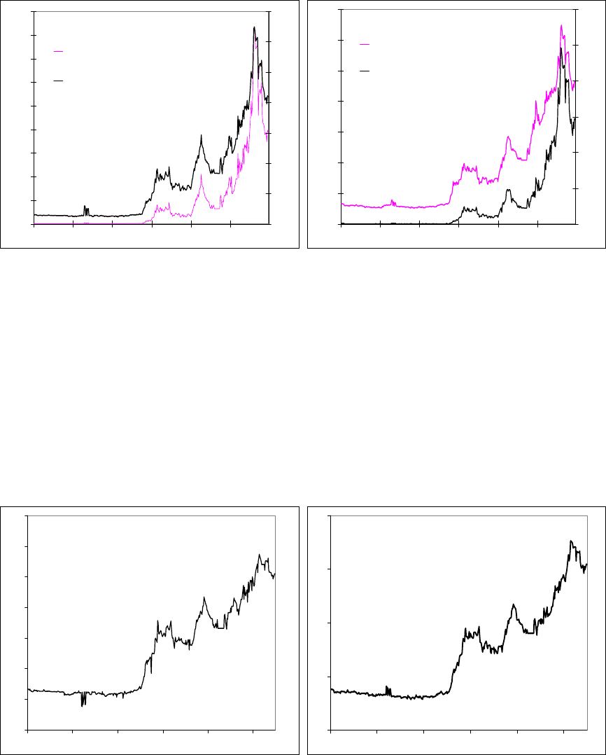
• The conditional resilience factor (RF) suggests that Singaporean banks are resilient

to an adverse systemic event. Among the Singaporean banks, one stands out as more

resilient (Figure I.4) and the other two banks demonstrate almost identical resilience,

confirming the finding from the DDMs that these two banks are becoming

increasingly interlinked. Among the regional banks in the sample, one bank stands

out as less resilient (Figure I.4).

Probability of Default over one year of a bank in a row, conditional on the default of a bank in a column.

Figure I.4. Resilience Factor

Singaporean banks Singaporean and Regional banks

0.1

0.2

0.3

0.4

0.5

0.6

0.7

0.8

0.9

12/1/06 3/1/07 6/1/07 9/1/07 12/1/07 3/1/08

Sing.bank 1

Sing.bank 2

Sing.bank 3

0.3

0.4

0.5

0.6

0.7

0.8

0.9

12/1/06 3/1/07 6/1/07 9/1/07 12/1/07 3/1/08

Sing.bank 2 Sing.bank 3 Sing.bank 1

Reg.bank 1 Reg.bank 2 Reg.bank 3

• Finally, the conditional systemic relevance factor (SRF) has been very similar for all

the banks. However, its magnitude goes down when the group of regional banks is

also taken into account (Figure I.5), most likely reflecting diversification gains.

Figure I.5. Systemic Relevance Factor

Singaporean banks Singaporean and Regional banks

0.05

0.1

0.15

0.2

0.25

0.3

0.35

12/1/06 3/1/07 6/1/07 9/1/07 12/1/07 3/1/08

Sing.bank 2

Sing.bank 3

Sing.bank 1

0.00

0.05

0.10

0.15

0.20

0.25

12/1/06 3/1/07 6/1/07 9/1/07 12/1/07 3/1/08

Sing.bank 2

Sing.bank 3

Sing.bank 1

Reg.bank 1

Reg.bank 2

Reg.bank 3

D. Concluding Remarks

10. This chapter provides an indicative assessment of the vulnerability of

Singapore’s banking system. The methodology builds on market indicators to derive

measures of banking system stability and can be extended to perform stress testing of the

banking system. In addition, the methodology provides technical improvements over other

methods to assess financial stability. For example, the estimated measures of vulnerability

account for time-varying dependencies among various banks. Thus, they go some way

toward capturing dynamic interdependencies among banks during times of financial distress.

11. Although the results need to be interpreted with care, overall they point to two

main findings:

• Ripple effects from the global credit crisis have been felt, but overall resilience of

Singapore’s banking system remains strong; and

• Regional bank integration appears to have an ambiguous impact, as diversification

gains may counter the opening up of addition channels for financial contagion. This

said, sample selection may also play a part in shaping this result.

References

Diebold, F., J.Hahn, and A.Taylor, 1999, “Multivariate Density Forecast Evaluation and

Calibration in Financial Risk Management: High-Frequency Returns on Foreign

Exchange,” The Review of Economics and Statistics, vol. 81, n. 4, pp.661-73.

Goodhart, C. and M. Segoviano, 2008, “Banking Stability Index,” IMF Working Paper,

forthcoming.

Monetary Authority of Singapore, 2007, “Financial Stability Review,” Singapore.

Segoviano, M., 2008, “The CIMDO-Copula: Robust Estimation of Default Dependence

under Data Restrictions,” IMF Working Paper, forthcoming.

Segoviano, M., 2006a, “The Conditional Probability of Default Methodology,” Financial

Market Group, London School of Economics, Discussion Paper 558.

II. THE EFFECTS OF MONETARY POLICY IN SINGAPORE

Singapore’s monetary policy is unique. It uses the exchange rate as an intermediate target to

achieve low inflation and sustainable growth. Over the past year, rising inflation and

slowing growth have posed challenges to the conduct of monetary policy. In this paper we

seek to understand better the impact of monetary policy on inflation and output using

structural vector autoregressions (SVAR). According to the empirical model, a

contractionary monetary policy shock (identified as a nominal effective exchange rate

appreciation) has powerful effects on both output and prices, providing support for the

exchange rate-centered monetary framework.

A. Introduction

1. Singapore manages its exchange rate against an undisclosed basket of

currencies. The Monetary Authority of Singapore (MAS) sets the rate of change of the

nominal effective exchange rate (NEER)—its intermediate target—to achieve low inflation

and sustainable growth. This framework has been in place since 1981 and over this period

annual inflation has been 1¾ percent (on average), while GDP growth has averaged

7 percent. Unemployment has also been remarkably low, at less than 3 percent during

1987–2007.

2. Starting in mid-2007, inflation has risen sharply—reaching almost 7 percent in

the first quarter of 2008—while growth has remained relatively strong. Several factors

have been in play, including a 2 percentage point increase in the sales tax (July 2007), a

sizable upward reassessment of property values (January 2008) and, more recently, spikes in

global commodity prices. In response, the MAS tightened monetary policy in October 2007

(steepening the slope of the exchange rate band) and April 2008 (recentering the band),

despite flagging external demand. Given Singapore’s exceptional trade openness, the current

environment poses challenges to Singapore’s exchange rate-centered policy framework.

3. This paper sheds light on Singapore’s unique monetary transmission

mechanism. It follows a well-established literature on estimating the effects of monetary

policy using structural vector autoregressions (SVARs). The paper uncovers powerful effects

of the exchange rate on output and inflation, supporting the rationale for the exchange rate-

centered monetary framework. Section B provides an overview of inflation developments in

Singapore, in particular its persistence and correlation with the nominal effective exchange

rate. Section C motivates the main assumptions underlying the SVAR. Section D presents the

main empirical results and briefly discusses alternative specifications, focusing on the impact

of monetary policy shocks on output and inflation. Section E concludes. The data and

technical estimation details are presented in the Annex.

Prepared by Roberto Guimaraes-Filho.

B. Inflation in Singapore: Some Stylized Facts

4. As noted above, inflation in

Singapore has been remarkably low and

stable but has recently picked up

significantly, reaching a 26-year high in

Q4 2007. The recent spike marks a

deviation from a declining trend. Inflation

has generally been trending downward

since the beginning of the1980s, averaging

2½ percent in the 1980s, 1¾ percent in the

1990s, and just over 1 percent during

2000–2007. With the exception of the

early 1980s, the volatility of inflation has

been generally low—ranging between 1 to 2 percent. Volatility has gone up since the second

half of 2007 on the wake of rising inflation.

5. Inflation has only been mildly

persistent over the last two decades. As

measured by the half-life of shocks from

simple univariate autoregressive (AR)

models, shocks to inflation have been

relatively short lived.

The empirical

model estimated for quarterly inflation is

an AR(1) or AR(2), depending on the sub-

sample.

The sum of the AR coefficients is

about 0.5–0.6, indicating that the half-life

of inflation shocks is about 1–1½ quarter.

6. Inflation in Singapore is

correlated with both the nominal

effective exchange rate and output. The

contemporaneous correlation between quarterly inflation and the NEER is relatively high at

The estimated degree of persistence at time t reflects what inflation is expected to be at time t + s, conditional

on all the present and past inflation up to time t.

The model is chosen according to the Bayesian information criterion. Low-order autoregressive dynamics are

present in the data, with one lag (or two, depending on the effective estimation sample) providing a good fit.

This is much lower than the estimated persistence calculated by Reis and Pivetta (2007) using post-WWII U.S.

data.

-20

-10

1980 1985 1990 1995 2000 2005

DNEERQ INFQ

CPI and NEER

(q/q change, in percent)

Inflation and Inflation Volatility

(annual, in percent)

-4

-2

Jan

-80

-82

Jan-84

Jan

-8

Jan

-88

Jan-90

Jan

-9

Jan

-94

Jan-96

Jan-98

Jan

-0

Jan-02

Jan-04

Jan

-0

Jan-08

-4

-2

Volatility

minus 0.4, suggesting that NEER appreciations tend to occur in tandem with lower inflation.

Granger predictability tests reveal that inflation Granger-causes the NEER, but the evidence

that the NEER causes inflation is weaker and not statistically significant. This suggests that

while monetary policy (captured by NEER changes) responds to inflation shocks rather

quickly, the pass-through from the exchange rate to inflation may be low and that the effect

of the NEER on inflation may operate with a long lag. Consistent with a Phillips curve

relationship, inflation is positively correlated with deviations of output from its trend.

C. Data and Empirical Model

7. The data are quarterly and span the period 1979–2007. The variables included in

the SVAR are the consumer price index (CPI), real GDP, the NEER, the domestic 3-month

nominal interbank interest rate (SIBOR), money aggregates (M1 and M2), and foreign

variables. The latter includes the “world” oil price (average from the IMF’s WEO), a trade-

weighted foreign GDP, and the 3-month LIBOR. In the case of GDP and CPI, the series are

seasonally adjusted. The data series are shown in the Annex.

8. The SVAR methodology is applied to identify monetary policy shocks and

simulate their impact on output and inflation. The baseline identification assumption is

adapted from Kim and Roubini (2000). They present a nonrecursive identification scheme

that generate hump-shaped response of output to a contractionary monetary policy shock and

has been widely used.

One of the main departures from Kim and Roubini (2000) is that the

NEER substitutes for the short-term interest rate in the policy reaction function. More

specifically, the SVAR model in this paper assumes that the model economy can be

represented by:

011

...

ttptpt

ykBy By u

−−

+++ +

where ][

tttttt

oil

ineermpxipy = is the n x 1 data vector containing the oil (or

commodity) price index (p

oil

), foreign interest rate (i*), real GDP (x), domestic CPI (p),

monetary aggregate (m), NEER, and domestic interest rate (i); k is a vector of constants, B

an n x n matrix of coefficients (with k = 1, ..., K), and u

is a white-noise vector of structural

shocks. All variables enter the VAR in natural logarithms.

9. The SVAR approach is well-suited to the analysis of monetary policy effects in

Singapore. One of the SVAR main advantages is its simplicity and the fact that it does not

This result is robust to at least two different measures of the trend (i.e., applying the HP and band-pass filters).

Other identification schemes are applied to assess the robustness of the results. The recursive identification of

Eichenbaum and Evans (1995) and the sign approach proposed by Uhlig (2005) are briefly discussed below.

impose potentially restrictive assumptions about behavioral relationships and the dynamics of

the economy. In the case of Singapore, the same monetary policy regime since the early

1980s provides a relatively long sample to identify monetary policy shocks without concerns

about structural breaks typically associated with changes in the policy regime.

10. The following contemporaneous restrictions are imposed to identify the

structural shocks (the details and the associated matrix are presented in the Annex):

• The commodity price index is exogenous with respect to all the variables in the

system; in contrast, the domestic interest rate (being a financial variable) is affected

by shocks to all other variables included in the VAR;

• The foreign interest rate and domestic output responds contemporaneously to the oil

price (or commodity prices) within a quarter, but the latter is not affected by the

former contemporaneously (zero restriction); as in Kim and Roubini (2000), firms

adjust output in response to policy shocks or financial market shocks with a lag;

• Domestic prices respond contemporaneously to oil price shocks and to output (the

second restriction can be relaxed without affecting the results);

• Money responds to domestic output and interest rates, consistent with standard money

demand theory. The restriction that the coefficient on the interest rate is zero may be

imposed without affecting the estimated impulse response functions; and

• The NEER responds to output, prices, the oil price, and domestic interest rates. The

inclusion of the oil price may account for the pre-emptive nature of monetary policy

as it responds to expected price pressures consistent with its medium-term orientation.

D. Main Findings

11. The main results from the SVAR are consistent with a strong effect of monetary

policy on output and prices. To evaluate the impact of the NEER on activity and the CPI,

the empirical model is used to estimate impulse-response functions. The results may be

described as follows:

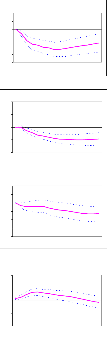
• A contractionary monetary policy shock is described as a NEER appreciation. The

appreciation is highly persistent and remains statistically significant up to 8 quarters;

No restrictions are imposed on the lagged structural parameters of the model.

• Consistent with the MAS’ own findings, contractionary monetary policy shocks have

strong effects on output. A NEER

appreciation shock lowers output (with a

hump-shaped impulse response

function)―the effect is economically and

statistically significant after 2 quarters and

peaks at 8 quarters. The lagged impact

justifies a forward-looking orientation of

monetary policy;

• A monetary policy contraction has a

persistent and strong negative effect on the

price level; the effect of the contractionary

shock on the CPI becomes economically

and statistically significant after 2 quarters

and peaks after 8 quarters;

• Underscoring the rationale for an

exchange rate-centered monetary policy

framework, the effect of an interest rate

increase on output is small and statistically

insignificant at the 5 percent level;

• Output shocks have a strong positive

impact on the CPI, as implied by a Philips

curve relationship (see also Parrado,

2004). The impact is strongest at

4–6 quarters and dissipates after

8–10 quarters as the effect of nominal and

other rigidities diminish;

• The NEER responds with relatively short

lags to shocks to the CPI and output. In

particular, the NEER appreciates in

response to increases in output (after

2 quarters) and the CPI (after 1 quarter).

The effect of the latter on the NEER is

generally small and is not statistically

significant at the 5 percent level. This is in

tune with an empirical characterization of

Response of CPI to NEER

(in percentage points)

-1.0

-0.5

0.0

0.5

1.0

12345678910111213141516

quarters

Response of CPI to output

(in percentage points)

-1.0

-0.5

0.0

0.5

1.0

1 2 3 4 5 6 7 8 9 10 11 12 13 14 15 16

quarters

Response of output to NEER

(in percentage points)

-2.0

-1.5

-1.0

-0.5

0.0

0.5

1.0

1 2 3 4 5 6 7 8 9 10 11 12 13 14 15 16

quarters

Response of output to interest rate

(in percentage points)

-2.0

-1.5

-1.0

-0.5

0.0

0.5

1.0

12345678910111213141516

quarters

monetary policy decisions in which the MAS targets the rate of change of the NEER

according to a Taylor-rule. Parrado (2004) and McCallum (2007) show that in fact a

Taylor rule for the NEER provides a good fit to the MAS’ policy reaction function.

• The effects of output (positive) and interest rate (negative) on monetary aggregates

(M1 or M2) is consistent with a well-behaved money demand curve; and

• As expected, the NEER and domestic interest rate respond strongly to foreign interest

rate shocks; also, domestic interest rates decline (on impact) following a NEER

appreciation.

12. Alternative identification schemes yield broadly similar results.

Applying a

slightly modified version of the Eichenbaum and Evans (1995) recursive assumptions, the

estimated VAR becomes

].[

tttttt

oil

ineermpxipy =

As noted above, the effect of an

interest rate shock on output is slightly stronger as well as the response of the NEER to CPI

shocks. Reversing the ordering of x and p or neer and i does not affect the qualitative results.

The results from imposing sign restrictions on the impulse responses (Uhlig, 2005) are also

consistent with those of the baseline model, but are less robust to the changes in the

underlying assumptions. For example, the negative response of the CPI to a contractionary

monetary policy shock is in line with results generated by standard monetary models, but the

impulse response (and its shape) depends largely on the assumed lagged effect of NEER

shocks on output.

E. Concluding Remarks

13. This paper assesses the effects of monetary policy on economic activity and

inflation. The findings suggest an important role for monetary policy in delivering low and

stable inflation, a salient feature of Singapore’s recent monetary history.

14. The results provide support for the exchange rate-centered monetary

framework. The main findings confirm that the effects of the interest rate shocks on output

In addition, there is no evidence of significant structural instability in the reduced-form VAR. For each

equation of the reduced-form VAR, Andrews’ sup-Wald test is applied to test jointly for the stability of all the

coefficients on the lags of a given variable. In this regard, the impulse response functions for the interest rate

and NEER based on a reduced form estimated over the 1991–2007 period are broadly similar to those reported

above, suggesting that there have been no major changes in the monetary transmission mechanism. (This may

change with the rising importance of domestic demand and interest rate-sensitive sectors). Interestingly, the

impact of interest shocks is larger (but is only marginally significant) when additional over-identifying

restrictions are imposed (see Annex).

The baseline recursive structure in Eichenbaum and Evans (1995) does not include the oil price but

incorporates the ratio of U.S. nonborrowed reserves to total (banking) reserves to identify the monetary policy

shocks.

and prices are significantly less important than those of the nominal exchange rate. In

addition, according to the estimated models, monetary policy can be empirically

characterized as a Taylor rule in which the NEER responds to output and inflation shocks.

The powerful effects of monetary policy combined with the credibility of the framework may

explain the relatively low inflation persistence.

Annex II.1. Estimation Details

15. The reduced form model is estimated with six lags in log-levels, except for the

domestic and foreign interest rate.

While all variables can be characterized as

nonstationary (or near-nonstationary as in the case of interest rates) according to standard

unit roots tests, most findings are robust to first differencing and inference can still be

conducted with the estimated model in levels (Canova, 2007, page 125). The structural model

can be rewritten in reduced form as:

...

ttptpt

ycCy Cy e

−−

+++ +

where

0tt

eBu

−

= is also white-noise vector process, with variance-covariance matrix given

,)(

′

−−

BDB where D is the variance-covariance matrix of the structural shocks. The

matrix

can be rewritten as

= 'ADA where D is diagonal. In this case, since

uAe

−

= ,

with A =

−

, then E(

′

) =

(())

EAee A

−−

′

()()AADAA

−−

′

= D, i.e., the vector u

orthogonal and can now be interpreted as “structural” shocks.

In practical terms,

identification amounts to imposing restrictions on the matrix

−

that orthogonalizes the

reduced form errors, eliminating their contemporaneous correlation.

A widely used

identification scheme is the recursive ordering (Cholesky decomposition) proposed by Sims

(1980), which assumes that A has a lower triangular structure. This is equivalent to a

hierarchical ordering of the variables, with the most exogenous variable ordered first.

16. Statistical inference can be conducted directly based on the estimated log-

likelihood. If there are n* estimated parameters in B

, the number of over-identifying

restrictions (r) is given by (( 1)/2) *rnn n=− −.

The test for over-identifying restrictions is

based on the maximized value of the log-likelihood and has a chi-square distribution with r

degrees of freedom.

The estimated reduced form has 4 lags and a time trend also yields a good fit, with the reduced form passing

the standard specification tests for autocorrelation and heteroskedasticity. Regarding the normality of the

residuals, there is some excess kurtosis as indicated by the Jarque-Bera test. The structural parameters are

estimated by maximum likelihood, but it may also be estimated by solving the nonlinear system given by

()BDB

−−

′

Ω=

Since e = B

-1

u and u = A

-1

e, the equality A = B

-1

follows immediately.

Alternatively, note that the matrices B

and D cannot have more unknowns than

. In this case, since D has n

parameters (it is diagonal) and

has n(n+1)/2 parameters (it is symmetric), this constrains B

to have at most

n(n-1)/2 free parameters.

(continued)

Identifying Restrictions

17. The restrictions described in the main text can be written as:

⎥

⎦

⎤

⎢

⎣

⎡

⎥

⎦

⎤

⎢

⎣

⎡

⎥

⎦

⎤

⎢

⎣

⎡

⎥

⎦

⎤

⎢

⎣

⎡

neer

poil

oil

neer

aaaaaa

aaaa

aaa

***

767574737271

67646361

575453

4341

)(

100

0100

00010

000010

000001

0000001

where

() ( )

LBL

∑

is a matrix polynomial in the lag operator (L) and u

is the vector of

“structural” shocks. In this case, the over-identifying restrictions test is distributed as a

chi-square with four degrees of freedom. For instance, according to the model above, the

empirical policy reaction function is given by:

tttxtt

uyLByaxaneer ++

′

+−=

−

)(

where the impact of output shocks on the NEER is given a

, and

−

′

is the vector of

coefficients excluding that on x. In this baseline specification there are four over-identifying

restrictions. Additional zero restrictions are also imposed on a

, a

and a

. In some cases,

the impact of the interest rate on output is larger but is only marginally significant (e.g., when

only a

= 0 is imposed).

The standard errors of the impulse responses are calculated by Monte Carlo simulation. They are broadly

similar to the probability bands are calculated from a Bayesian method that employs a Gaussian approximation

to the posterior of the matrix A (recommended by Sims and Zha (1999) for overidentified models).

References

Canova, Fabio (2007). Methods for Applied Macroeconomic Research. Princeton University

Press.

Eichenbaum, Martin and Evans, Charles (1995). “Some Empirical Evidence on the Effects of

Monetary Policy Shocks on Exchange Rates

,” Quarterly Journal of Economics,

110(4), 975-1009.

Kim, Soyoung and Roubini, Nouriel, (2000). “Exchange rate anomalies in the industrial

countries: A solution with a structural VAR approach,” Journal of Monetary

Economics, 45(3), pages 561-586.

McCallum, Bennett (2007). “Monetary Policy in East Asia: the case of Singapore,” IMES

Discussion Paper 2007 E10.

Parrado, Eric (2004). “Singapore’s Unique Monetary Policy Framework: How Does It

Work?” IMF Working Paper.

Reis, Ricardo and Pivetta, Frederic. (2007). “The Persistence of Inflation in the United

States,”

Journal of Economic Dynamics and Control, 31 (4), 1326-1358.

Sims, Christopher, and Zha, Tao (1999). “Error Bands for Impulse Responses,”

Econometrica, 67 (5), 1113-1155.

Uhlig, Harald (2005). “What Are the Effects of Monetary Policy? Results from an Agnostic

Identification Procedure,” Journal of Monetary Economics, 52 (2), 190-212.

III. EFFECTIVENESS OF FISCAL POLICY IN SINGAPORE

Singapore’s policy makers have often relied on fiscal policy to counter the impact of adverse

external shocks. Against the background of the current uncertain external environment, this

chapter analyze the effectiveness of fiscal policy in managing the economic cycle in

Singapore. Empirical results based on a structural autoregression framework suggest that

fiscal policy can be used as a counter-cyclical tool, but that the impact of fiscal policy is

relatively short-lived and cumulatively small. This may reflect a number of factors, including

the absence of credit-constrained economic agents, a high propensity to save among

households, the use of quasi-fiscal measures not captured in budgetary data, a monetary

focus on price stability, and leakages due to the openness of the economy.

A. Introduction

1. The effectiveness of fiscal policy as a counter-cyclical tool is the subject of a

longstanding debate among economists.

Supporters of an active role for fiscal policy

suggest that economies lack an efficient mechanism to return to full potential. Critics, on the

other hand, argue that economic agents could offset the impact of fiscal policy on aggregate

demand through changes in their savings behavior. A middle-of-the-road view holds that

fiscal policy can be effective provided certain conditions hold, including sound

macroeconomic fundamentals, nominal wage and price stickiness, imperfect competition,

and/or economic agents with finite horizons and liquidity constraints.

Singapore has often used fiscal policy to counter adverse external shocks. In the

aftermath of the Asian crisis (1998), the bursting of the tech-bubble (2001), and the SARS

shock (2003), the authorities used fiscal policy to help cushion the impact on economic

activity and vulnerable groups. The fiscal counter-measures focused on relief for both

businesses and households, including through tax incentives, tax credits, transfer payments,

and various rebates on housing and utilities.

3. In the context of the current uncertain external environment, the chapter

analyzes empirically the effectiveness of fiscal policy in Singapore. Fiscal multipliers are

estimated using a structural vector autoregression (SVAR) framework. The chapter is

organized as follows: Section B looks at the cross-country evidence on the effectiveness of

fiscal policy; Section C presents the empirical approach (elaborated in the Annex) and results

for Singapore; and Section D concludes.

Prepared by Leif Lybecker Eskesen

See IMF World Economic Outlook, April 2008.

B. Cross-country Evidence on the Effectiveness of Fiscal Policy

4. The question of the effectiveness of fiscal policy is ultimately empirical. There is a

vast literature on this topic. Studies generally support the role for counter-cyclical measures,

but evidence on the size of fiscal multipliers is uneven:

• Event-studies give mixed results. The 2001 income tax rebates in the United States

are generally considered to have been effective in boosting domestic demand,

although the impact on output was relatively small with multipliers well below 1

(Shapiro, et al. (2002, 2003)). The 1995 stimulus package in Japan is estimated to

have been successful in the short term, but it did not have a lasting impact on

economic activity (Posen (1998), Mühleisen (2000)). However, Finland’s response to

the 1991 output shock, by letting automatic stabilizers operate fully, is considered to

have been largely ineffective because it raised concerns about fiscal sustainability

(Corsetti and Roubini (1996)).

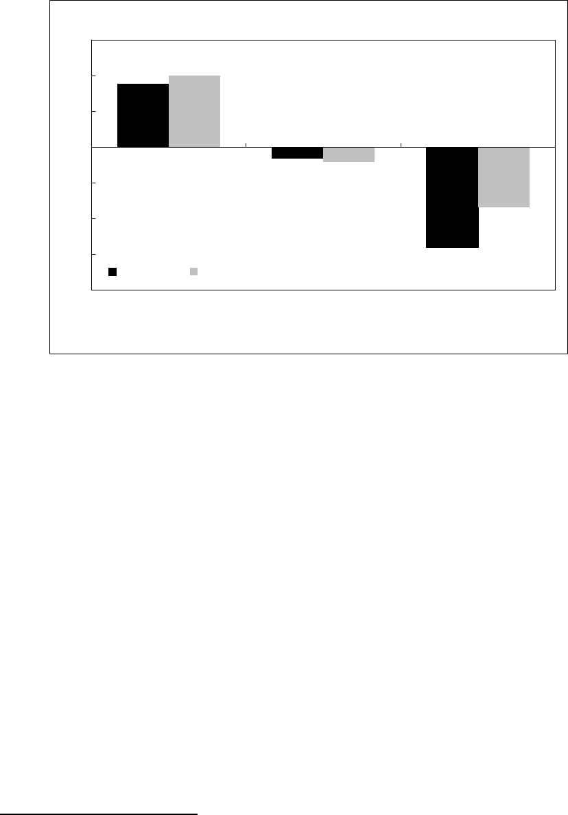
• Studies on advanced economies using vector autoregressive (VAR) methods

conclude that fiscal multipliers have declined over time and, in some cases, may even

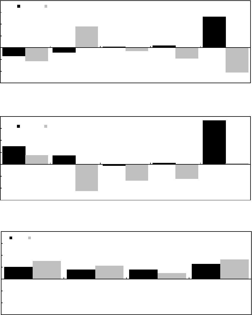
have been negative (see Perotti (2005) for an overview). These results (Figure III.1),

which differ widely across countries, likely reflect: (i) more leakage through the trade

channel due to increased openness of economies; (ii) a decline in the share of

liquidity constrained households due to better access to credit; and (iii) a sharper

focus of monetary policy on price stability.

• Estimates from macro models, on the other hand, show that fiscal policy can be quite

effective (Figure III.1).

Impact multipliers are in the range of 0.3 to 1.2 percent upon

impact. Furthermore, expenditure measures appear to have a larger effect than tax

measures (Hemming and others 2002, Botman 2006). However, the size of the

estimated multiplier depends on assumptions about parameters such as labor supply

elasticities and the pervasiveness of liquidity constraints.

5. Generally, the cross-country evidence suggest that the success of fiscal policy is

contingent on a number of factors. First, the fiscal response needs to be well-timed. This

will tend to increase the effectiveness of fiscal policy in countries with short implementation

lags and/or large automatic stabilizers (the latter being the first line of defense). Second,

strong fundamentals, including macroeconomic stability and fiscal sustainability, will

strengthen multiplier effects by lowering any possible offsets from precautionary savings.

Finally, fiscal measures need to be well-targeted to ensure the largest possible demand

impact.

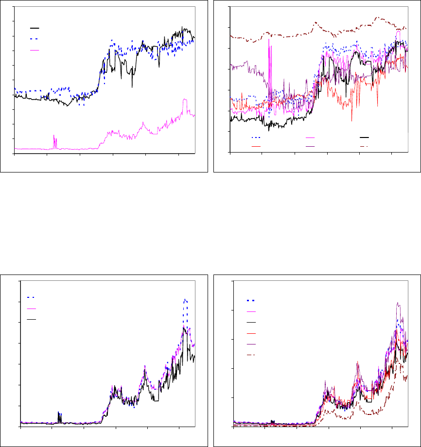
Figure III.1. Fiscal Multipliers from SVAR and Macroeconometric Models

- Cross-country Evidence

Source: Perotti (2005).

Fiscal Multipliers from SVAR Models: 1 Percent of GDP Increase in Spending

(Cumulative GDP response at 12 quarters over different time periods)

-3

-2

-1

ustralia Canada Germany United Kingdom United States

1960-1980 1980-2001

Fiscal Multipliers from SVAR Models: 1 Percent of GDP Tax Cut

(Cumulative GDP response at 12 quarters over different time periods)

-3

-2

-1

ustralia Canada Germany United Kingdom United States

1960-1980 1980-2001

Fiscal Multipliers from Macroeconometric Models: 1 Percent of GDP Spending Increase

(Cumulative GDP response at 4 and 8 quarters)

-3

-2

-1

Euro Area Germany United Kingdom United States

1 year 2 years

C. Effectiveness of Fiscal Policy in Singapore

Empirical Approach

6. VAR methods are standard in monetary policy analysis, but have only recently

been applied to fiscal policy. This chapter does so by applying the SVAR methodology

developed in Blanchard and Perotti (2002).

Intuitively, this methodology utilizes the (“inside”) lags in fiscal policy to identify

discretionary structural fiscal shocks and their impact on economic activity:

• Assuming that discretionary fiscal policy decisions take time to be implemented

(because of political and legislative requirements), the short-term (i.e., within one

quarter) reaction of fiscal variables to current economic developments only reflect

“automatic” responses defined by existing laws and regulations.

•

Fiscal developments adjusted for these automatic/cyclical responses are, therefore,

assumed to represent discretionary structural fiscal policy shocks.

•

In simulations, these structural shocks are used to quantify the response of real

economic variables to discretionary fiscal policy. In the case of Singapore, the focus

is on private domestic demand, in part to abstract from first-order leakages.

A technical description of the methodology is presented in the Annex to this chapter.

Empirical Results

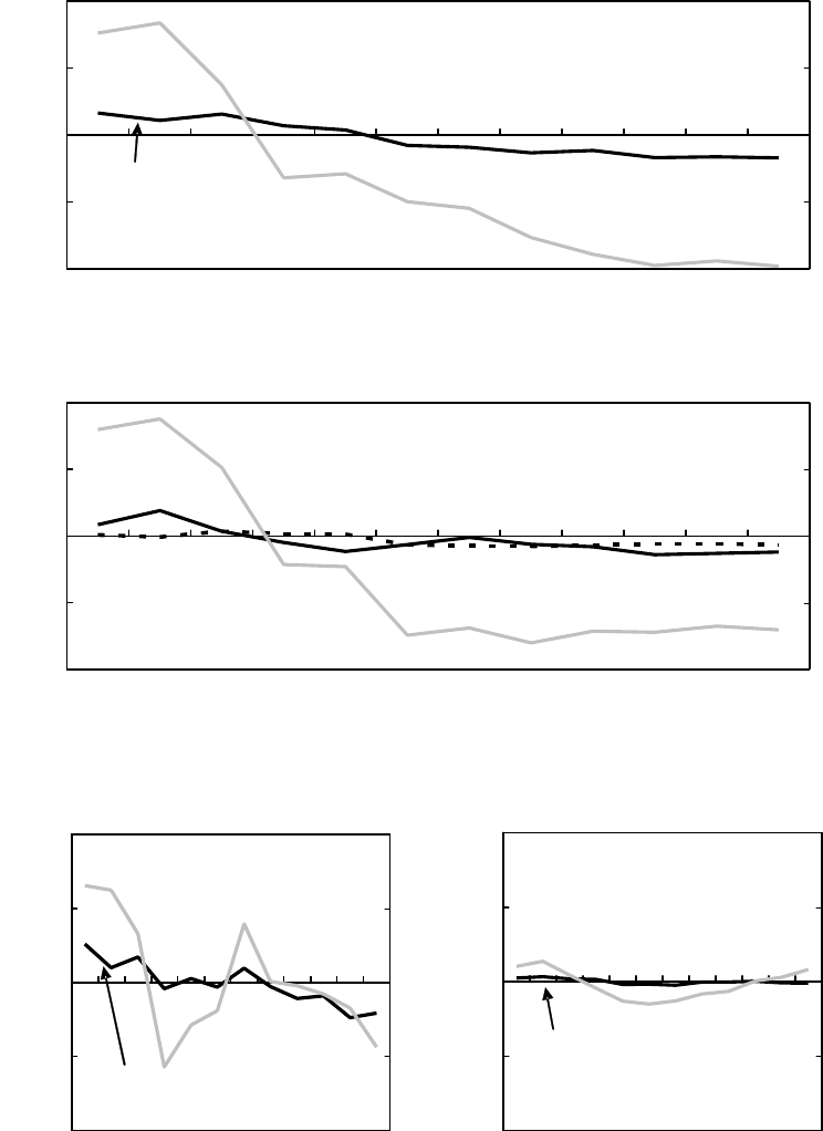
8. Empirical results suggest that discretionary fiscal policy can have an immediate

impact on private domestic demand and play a role as a counter-cyclical tool. However,

the impact drops off quickly and eventually turns negative (Figure III.2 and III.3), leaving the

cumulative effect relatively small compared to other countries. The estimated impulses are

generally not significant past the fourth quarter. By aggregate demand component, the

estimated impulse response functions (not shown here) suggest fiscal policy appears to have

a larger impact on private investment than on private consumption. This may reflect a high

precautionary savings-motive among Singaporean households and a government strategy of

partly focusing discretionary measures on strengthening household savings.

Changes in revenues are estimated to have the largest impact-effect on private

demand, but that impact fizzles out quickly. This is in contrast to results obtained for a

number of other industrial countries, which tend to show a larger multiplier for expenditure

measures. However, the puzzle could in part be explained by the narrower definition of

government expenditure used here, which excludes key income transfers for lack of quarterly

data.

Figure III.2. Singapore: Fiscal Multipliers in Singapore - SVAR Results

Source: Staff estimates

Fiscal Stimulus: Impact on Domestic Demand over 12 Quarters - Model 1

(One percent innovation in fiscal variable)

Expenditure

Revenues

-1.0

-0.5

0.0

0.5

1.0

1 2 3 4 5 6 7 8 9 10 11 12

-1.0

-0.5

0.0

0.5

1.0

Fiscal Stimulus: Impact on Domestic Demand over 12 Quarters - Model 2

(One percent innovation in fiscal variable)

Current Expenditure

Capital Expenditure

Revenue

-1.0

-0.5

0.0

0.5

1.0

1 2 3 4 5 6 7 8 9 10 11 12

-1.0

-0.5

0.0

0.5

1.0

Fiscal Stimulus: Impact on Domestic Demand and Inflation over 12 Quarters - Model 3

(One percent innovation in fiscal variable)

Impact on domestic demand

Revenue

-1.0

-0.5

0.0

0.5

1.0

1 2 3 4 5 6 7 8 9 10 11 12

-1.0

-0.5

0.0

0.5

1.0

Expenditure

Impact on inflation

Revenue

-1.0

-0.5

0.0

0.5

1.0

1 2 3 4 5 6 7 8 9

10 11 12

-1.0

-0.5

0.0

0.5

1.0

Expenditure

10. Among expenditure components, the simulations show that changes in

government current spending provides more stimulus than changes in public

investment. Indeed, the estimates for investment multipliers are generally insignificant. This

may reflect some crowding out of private investment activity.

11. A fiscal expansion has a positive but limited impact on inflation. The largest

impact is related to changes in taxes, which is consistent with the estimated larger impact on

private demand (and hence inflation pressures) from changes in government revenues.

Government spending, on the other hand, does not appear to have a significant impact on

prices.

D. Concluding Remarks

12. Singapore’s large fiscal reserves provides ample scope to use fiscal policy to

counter adverse external shocks. Given Singapore’s relatively small automatic stabilizers, a

counter-cyclical response—when needed—would have to be primarily discretionary.

However, the short fiscal lags allow for a fast response to changing economic conditions. In

an uncertain external environment such as today’s, this flexibility provides some insurance

against further negative spillovers from a more pronounced deterioration in the global

economy.

Singapore does not have a comprehensive unemployment benefit scheme and corporate taxes are assessed

based on previous year’s income.

Figure III.3: Cumulative Multipliers - Model 1

- Cumulative impact on private demand from a fiscal expansion of 1 S$

-2.0

-1.5

-1.0

-0.5

0.0

0.5

1.0

1.5

4 quarters 8 quarters 12 quarters

Expenditure Revenues

Note: The cumulative multiplier at a given quarter equals the ratio of the cumulative response of private demand and the

cumulative response of the fiscal variable.

13.

Preliminary results suggest that fiscal policy in Singapore can serve as a tool for

demand management, but cumulative fiscal multipliers are generally found to be small.

This may reflect a number of factors, including:

•

The absence of credit-constrained households, leading to a somewhat lower

consumption response, on the margin, to changes in disposable incomes;

•

A high propensity to save among households—possibly, in part, reflecting the

absence of a more comprehensive social safety net;

•

The use of nonbudgetary measures, including changes in contributions to the

mandatory public savings scheme (CPF), to stimulate activity. These are not captured

in the fiscal variables used in this study;

•

Strong monetary focus on price stability, which may partly offset the effect of fiscal

stimulus;

•

Significant leakages through trade as well as remittances (nonresident workers

account for around 30 percent of the labor force), which may weaken the dynamic

interrelations between domestic demand components.

14. This analysis could be expanded. It could be useful in future research to analyze the

impact of more disaggregated fiscal measures on private demand and its sub-components,

which could help strengthen fiscal design. A study of the impact of income transfers would

be particularly desirable, since they are often used as a counter-cyclical as well as

redistributive tool. Finally, the results could be subjected to sensitivity analysis, including

with respect to the assumed expenditure and revenue elasticities. All these potential

extensions remain on the research agenda.

Annex III.1. Technical Description of the Fiscal SVAR Framework

The basic VAR specification is:

(1) z

= Γ(L)z

t-1

+ u

where z

is a nx1 vector of endogenous variables, Γ(L) is a nxn matrix of lag polynomials in

the lag operator L and u

is a nx1 vector of reduced-form innovations, which are independent

and identically distributed. The relation between the reduced-form innovations u

and the

objects of ultimate interest, the structural shocks v

, can be represented as:

(2) Au

=Bv

where the nxn matrices A and B describe (i) the instantaneous relation between the variables

and (ii) the linear relationship between the structural shocks and the reduced form residuals,

respectively. The structural shocks are assumed to be orthogonal, which allows for impact

analysis of an isolated shock. The structural form of the VAR can be obtained by multiplying

(1) by A and using the relation defined in (2):

(3) Az

=AΓ(L)z

t-1

+Au

=AΓ(L)z

t-1

+Bv

Solving (3) for z

yields the structural specification:

(4) z

=[I−Γ(L)L]

−1

Where I is a nxn identity matrix. In the simplest specification used in this study,

=[y

] consists of three variables for Singapore: real private domestic demand, y

; real

government expenditure (consumption and investment), e

; and real current government

revenue, r

The data used are seasonally adjusted and at a high frequency (quarterly) in

order to identify the structural shocks. The VAR is estimated in log levels with a constant,

time dummies, and G7 growth added as exogenous explanatory variables. The number of

lags chosen is five as suggested by Akaike and other information criteria.

Quarterly data for special transfers were unfortunately not available and are, therefore, not included in the

expenditure data.

The models specified in this paper are robust to alternative specifications and residuals do not appear to suffer

from autocorrelation. Tests for normality of error terms suggest there is not an issue with skewedness, but they

cannot reject the hypothesis that there may be an issue with kurtosis.

Estimation basically proceeds in four steps. In the

first step, the reduced form VAR is

estimated, yielding the reduced form residuals

[

]

uuuu = :

(5)

vuuu ++=

αα

(6)

vvuu ++=

βα

(7)

vvuu ++=

βα

As suggested by Perotti (2005), the innovations in

u and

u can be thought of as linear

combinations of three types of shocks: (i) the automatic or cyclical response of expenditures

and revenues to innovations in private domestic demand; (ii) the systematic response of fiscal

policy to same-period macro shocks; and (iii) discretionary fiscal policy shocks, which are

the

structural shocks we are interested in identifying. This gives the following representation

of the reduced form residuals for the fiscal variables:

(8)

vvuu ++=

βα

(9)

vvuu ++=

βα

where

v and

v are the structural shocks to government expenditure and revenues,

respectively. Since fiscal policy is implemented with a lag, systematic discretionary

responses to macro shocks (i.e., item (ii) in the previous paragraph) are absent in quarterly

data. As a consequence, the coefficients

and

in (8) and (9) only capture the

automatic/cyclical response of fiscal variables to economic activity.

Given that the reduced form residuals are correlated with the structural shocks, exogenous

elasticities are used to estimate the automatic/cyclical response of the fiscal variables.

With

these, one can then construct the cyclically adjusted fiscal shocks, which constitutes the

second step of the estimation procedure:

Representation of the exogenous variables are excluded here to allow for a simplistic illustration of the model.

For Singapore, the elasticity of expenditures with respect to changes in economic activity is assumed to be

close to zero within the quarter, as commonly assumed in many other empirical studies. The elasticity of

revenues is estimated at around ½ percent within the quarter. The relatively low number partly reflects that

corporate taxes are based on past year’s rather than contemporaneous earnings, leaving taxes less responsive to

contemporaneous changes in economic activity. While the parameterization is plausible, the magnitude has

implications for the estimated multipliers.

(10)

adje

vvuuu +=−≡

βα

(11)

adjr

vvuuu +=−≡

βα

In the

third step, the structural fiscal shocks are determined. Assuming that structural

revenue shocks have no impact on structural spending shocks, (10) and (11) become:

(12)

adje

vu =

(13)

adjr

vvu +=

The structurally adjusted expenditure shock is, consequently, equal to the cyclically adjusted

expenditure shock. With this, it is now possible to estimate the response of revenues to

structural expenditure shocks,

, using simple OLS.

In the

fourth and final step, the coefficients in the equation for private domestic demand

residuals (5) can be determined. Combined, the four steps, which are effectively done

simultaneously, allow us to estimate the

A and B matrices presented in (2):

⎥

⎦

⎤

⎢

⎣

⎡

⎥

⎦

⎤

⎢

⎣

⎡

⎥

⎦

⎤

⎢

⎣

⎡

⎥

⎦

⎤

⎢

⎣

⎡

−

010

001

βα

αα

In turn, these are used to compute the structural impulse responses of private domestic

demand to discretionary expenditure and revenue shocks.

References

Baxter, Marianne and Robert G. King (1993), “Fiscal Policy in General Equilibrium,”

American Economic Review, American Economic Association, vol. 83(3),

pages 315–34, June.

Bayoumi, Tamim (2001), “The Morning After: Explaining the Slowdown in Growth in the

1990s,” in T. Bayoumi and Ch. Collyns (eds.) Post-Bubble Blues-How Japan

Responded to Asset Price Collapse, IMF 2000.

Blanchard, Olivier and Roberto Perotti (2002), “An empirical characterization of the

dynamic effects of changes in government spending and taxes on output,” Quarterly

Journal of Economics 117, 1329–1368.

Blinder, Alan (2004), “The Case Against the Case Against Discretionary Fiscal Policy,”

CEPS Working Paper No. 100.

Corsetti, Giancarlo and Nouriel Roubini

(1996), “Budget Deficits, Public Sector Solvency and

Political Biases in Fiscal Policy: A Case Study of Finland,” Finnish Economic Papers,

Spring, v. 9, iss. 1, pp. 18–36.

De Castro Fernández, Francisco and Pablo Hernández de Cos (2006), “The economic effects

of exogenous fiscal shocks in Spain: a SVAR approach,” ECB Working Paper,

vol. 647. European Central Bank, Frankfurt.

Giavazzi, Francesco and Marco Pagano (1990), “Can Severe Fiscal Contractions be

Expansionary? Tales of Two Small European Countries,” NBER Macro Annual 5,

75–111.

Giordano, Raffaela, Sandro Momigliano, Stefano Neri, and Roberto Perotti (2007), “The

Effects of Fiscal Policy in Italy: Evidence from a VAR model,” European Journal of

Political Economy 23, 707–33.

Hemming Richard, Michael Kell, and Selma Mahfouz (2002), “The effectiveness of Fiscal

Policy in Stimulating Economic Activity—A Review of the Literature,” IMF working

Paper 02/208.

Heppke-Falk, Kirsten H., Jörn Tenhofen, and Guntram B. Wolff (2006), “The

macroeconomic effects of exogenous fiscal policy shocks in Germany: a

disaggregated SVAR analysis,” Discussion Paper, Series 1: Economic Studies,

41/2006, Deutsche Bundesbank.

International Monetary Fund (2008), “World Economic Outlook, April 2008.”

Johnson, David S., Jonathan A. Parker, and Nicholas S. Souleles (2004), “The Response of

Consumer Spending to the Randomized Income Tax Rebates of 2001,” The Wharton

School working paper, February 2004.

Kuttner, Kenneth and Adam Posen (2002), “Fiscal Policy Effectiveness in Japan,” Journal of

the Japanese and International Economies 16, 536–558

Linnemann, Ludger and Andreas Schabert (2003), “Fiscal Policy in the New Neoclassical

Synthesis,” Journal of Money, Credit and Banking, Vol. 35, No. 6, pp. 911–929.

Mühleisen, Martin (2000), “Too much of a Good Thing? The Effectiveness of Fiscal

Stimulus”, in: T. Bayoumi and Ch. Collyns (eds.), “Post-Bubble Blues-How Japan

Responded to Asset Price Collapse,” IMF 2000.

Perotti, Roberto, (2005), “Estimating the Effects of Fiscal Policy in OECD Countries,” CEPR

Discussion Paper 4842.

———, (2007), “In Search of the Transmission Mechanism of Fiscal Policy,” NBER

Working Paper 13143.

Posen, Adam (1998), “Restoring Japan’s Economic Growth,” Institute for International

Economics, Washington DC.

Shapiro, Matthew D. and Joel Slemrod (2003), “Consumer Response to Tax Rebates,”

American Economic Review, Vol. 93 (1), 381–396

——— (2002), “Did the 2001 Tax Rebate Stimulate Spending? Evidence from Taxpayer

Surveys,” NBER Working Paper 9308.