
1339681v1-THE EFFECTIVENESS OF FISCAL PO.DOC November 21, 2001 (1:46 PM)
The Effectiveness of Fiscal Policy in Stimulating Economic Activity
An Empirical Investigation
Emanuele Baldacci, Marco Cangiano, Selma Mahfouz, and Axel Schimmelpfennig
1
November 2001
Preliminary draft. Comments welcome
Abstract
Recent years have seen a revival of the debate about the role of fiscal policy in stimulating economic
activity. The empirical literature suggests that fiscal multipliers are typically positive but small, and
while there is some evidence of negative fiscal multipliers, there is no clear consensus on the
preconditions for such an outcome. However, most of the empirical evidence is for advanced
economies and the effectiveness of fiscal policy in emerging market economies, countries in
transition, and developing countries remains largely undocumented. This paper tries to fill this gap by
using data for a large number of countries, including developing countries and emerging market
economies, to examine whether some of the factors identified in the theoretical literature are indeed
important in explaining the effectiveness of fiscal policy in responding to a recession. The focus is on
episodes of recession and the associated fiscal policy response. Given the large number of countries
and episodes, and differences in the size and composition of fiscal responses, initial conditions, and
accompanying policies and developments, the paper explores three different and complementary
approaches to try to account for the interactions between fiscal policy and growth during recession
episodes: descriptive analysis, multidimensional statistical analysis, and standard regression analysis.
JEL Classification Numbers: C21, E62, E65, H30
Keywords: Fiscal policy, stabilization, recession, principal components and cluster analysis.
1
Paper to be presented at Second Annual Research Conference organized by the International Monetary Fund,
Washington DC, November 29-30, 2001. We thank Richard Hemming for his constant encouragement and
suggestions, Michael Kell for helpful comments, and Estella Macke for her excellent research assistance. The
usual disclaimer applies.
- 2 -
I. Introduction 3
II. Definitions and Data 4
A. Definitions.................................................................................................................4
B. Data ...........................................................................................................................5
III. Descriptive Analysis 7
A. Overview of Recession Episodes..............................................................................7
B. Fiscal Response During a Recession.........................................................................9
C. Fiscal Response and Economic Activity in a Recession.........................................12
Initial conditions ..............................................................................................13
Composition of fiscal policy............................................................................15
Accompanying policies....................................................................................16
D. Sensitivity Analysis.................................................................................................17
Sample..............................................................................................................17
Selection bias ...................................................................................................17
E. Preliminary Findings...............................................................................................18
IV. Exploratory Multidimensional Analysis 19
A. Rationale .................................................................................................................19
B. Principal Components Analysis..............................................................................20
C. Cluster Analysis ......................................................................................................22
D. What Have We Learned?........................................................................................30
V. Estimates of a Reduced-Form Equation 32
A. Methodology...........................................................................................................32
B. Specification Search and Results ............................................................................32
Specification strategy.......................................................................................32
Model 1: Regional dummy variables..............................................................33
Model 2: Cluster dummy variables..................................................................33
VI. Concluding Remarks 35
Figures
Figure 1. Number of Countries in Recessions, 1971-98............................................................8
Figure 2. Distribution of Cluster Centers by Selected Factors ................................................28
Figure 3. Distribution of Cluster Centers by Selected Factors ................................................29
Appendices
Appendix I. Variables, Definitions, and Data Sources............................................................37
Appendix II. Multidimensional Analysis: A Methodological Note.........................................40

- 3 -
I. I
NTRODUCTION
Recent years have seen a revival of the debate about the role of fiscal policy in stimulating
economic activity, particularly given the recessions in Asian crisis countries, the prolonged
slump in Japan and, more recently, the slowdown in the United States. Lane and others
(1999), while noting fiscal policy in the Asian crisis countries became increasingly oriented
toward supporting economic activity as the assessment of the economic situation was
changing, point to the questions that remain about the effectiveness of fiscal stimulus during
a crisis. Even if it is generally agreed that there are circumstances where fiscal policy cannot
be loosened (e.g. when fiscal imbalances or debt sustainability problems are the root causes
of the crisis), whether and when expansionary fiscal policy is effective in supporting activity
needs to be studied further.
There is a large literature on the effectiveness of fiscal policy in stimulating economic
activity in the short term—see Hemming, Kell and Mahfouz (2000) for a review. Economic
theory suggests that fiscal multipliers are more likely to be positive and large when
economies are relatively closed, there is considerable slack in productive capacity,
government debt is low, fiscal expansion focuses on spending, and there is an accompanying
monetary expansion. Fiscal multipliers will be smaller, and could turn negative, when debt
sustainability problems result in large risk premia on interest rates, consumers are Ricardian,
expectations intensify crowding out effects, or a fiscal expansion increases uncertainty. The
empirical literature suggests that fiscal multipliers are typically positive, but small, and while
there is some evidence of negative fiscal multipliers, there is no clear consensus on the
preconditions for such an outcome. However, most of the empirical evidence is for advanced
and mainly G3 economies. The effectiveness of fiscal policy in emerging market economies,
countries in transition, and developing countries remains largely undocumented.
2
This paper uses data for a large number of countries, including developing countries and
emerging economies, to examine whether there is any evidence that some of the factors
identified in the theoretical literature are indeed important in explaining the effectiveness of
fiscal policy in responding to a recession.
Following the approach initiated by Giavazzi and Pagano (1996) and Alesina and Perotti
(1997), the focus is on specific episodes, but in this case it is episodes of recession rather
than episodes of fiscal expansion or contraction, and the response of fiscal policy and its
effectiveness in connection with these episodes. There are two main reasons for focusing on
recession episodes. First, the question of whether fiscal policy is effective in stimulating
economic activity is particularly crucial and often raised when a country is experiencing a
recession or downturn. Second, the impact of fiscal policy on economic activity is likely to
2
One notable exception is Giavazzi, Japelli, and Pagano (2000).

- 4 -
be more visible in periods of slow growth, when there is a lot of slack in the economy and the
priority is to revive the economy.
Given the large number of countries and episodes, and differences in the size and
composition of fiscal responses, diversity of initial conditions, and accompanying policies
and developments, together with the complexity of channels through which fiscal policy may
affect economic activity, no single approach can extract all the relevant information from the
data. The paper therefore explores three different and complementary approaches to try to
account for the interactions between fiscal policy and growth during recession episodes:
simple descriptive analysis, multidimensional statistical analysis, and regression analysis.
The paper is organized as follows. Section II presents the definitions and the data used in the
rest of paper. Section III reports stylized facts about economic activity and fiscal policy
during recession episodes. Section IV summarizes the results of a multidimensional statistical
approach which partitions the recession episodes into groups with common characteristics.
Based on the insights provided by the descriptive and statistical analyses, Section V reports
on an econometric investigation aimed at testing more formally the relationship between
economic activity and fiscal policy in recessions. Section VI contains the main conclusions.
II. D
EFINITIONS AND
D
ATA
A. Definitions
The following definitions are used in the rest of the paper:
• A recession episode is defined as a single year or consecutive years in which real
GDP growth is more than one standard deviation below trend growth (defined as the
average growth for the country over the period 1970-1999).
• The fiscal response during a recession episode is measured by the difference between
the average fiscal balance in percent of GDP during the episode and before the
episode, multiplied by the length of the episode.
3
When this difference is negative,
there is an expansionary fiscal response.
• The severity of a recession is measured by the cumulative difference over a
recession episode between real GDP growth and trend growth.
4
This measure can be
broken down into average annual growth (relative to trend growth) during the
recession and the length of the recession.
3
Thus, if the fiscal deficit was 1 percent of GDP before the recession, and increased to 4 then 5 percent over a
two-year recession, the fiscal response would be -7 percent of GDP.
4
Thus if a country’s real GDP growth was -1 percent during two years of recession, while trend growth over
1970-1999 was 2 percent, the severity of the recession would be -6 percent.

- 5 -
• The effectiveness of fiscal policy is measured by the difference in growth outcomes
during recession episodes accompanied by an expansionary fiscal policy and episodes
accompanied by a contractionary fiscal policy. While not an exact measure of the size
of fiscal multipliers, this measure distinguishes whether they are positive or negative.
The correction for trend growth in defining and measuring the severity of a recession reflects
the view that differences in trend growth across countries—which are quite large in our
sample—reflect structural factors unrelated to the response of fiscal policy.
The use of the change in the actual fiscal balance to measure the stance of fiscal policy is
primarily dictated by the absence of data on structural balances for most of the countries in
the sample. The advantages of using the actual balance are that automatic stabilizers are
therefore part of the fiscal response and that it avoids making a contentious distinction
between the discretionary and automatic components of fiscal policy in a recession.
5
On the
other hand, since the actual balance is likely to be influenced by real GDP growth, it will be
necessary to account for possible endogeneity bias (see Sections III and V).
B. Data
One of the objectives of this study is to have as broad a coverage of countries and episodes as
possible. As a result, the choice of the variables used and the empirical strategy is largely
driven by data availability. The sample covers 168 countries over the period 1970-1999.
6
Annual data are largely derived from a number of IMF databases, complemented by World
Bank public debt data.
7
Countries are divided into six groups, based on the World Economic Outlook (WEO) country
classification: advanced economies (ADV), including newly industrialized Asian economies,
four groups of developing countries, Africa (AFR), developing Asia (ASIA), Middle East
(ME) and Western Hemisphere (WH), and countries in transition (CIT).
Although the theoretical literature suggests a long list of factors that may influence the
effectiveness of fiscal policy (see Box 1 in Hemming, Kell, and Mahfouz (2000)), many of
these (e.g. uncertainty, sensitivity of consumption and investment to interest rates) are
5
Determining what constitutes a discretionary policy action remains highly judgmental since any forms of
policy inaction can be viewed as a deliberate choice to maintain the status quo. For a discussion of this issue in
the context of the Asian crisis, see Box 2.5. “Fiscal balances in the Asian Crisis Countries. Effects of Changes
in the Economic Environment Versus Policy Measures,” in IMF, 1998.
6
For countries in transition, episodes prior to 1994 (transition period) are excluded.
7
A detailed presentation of data sources and variables is given in Appendix 1.

- 6 -
difficult to quantify for a large number of countries. The analysis is therefore limited to the
following factors:
8
Initial conditions:
• slack in the economy, measured by real GDP growth before the recession,
• openness, measured by the ratio of imports to GDP before the recession,
• exchange rate regime, measured by a dummy variable (flexible or fixed),
• debt sustainability, measured by the public debt to GDP ratio before the recession,
• financing constraints facing the government, measured by the fiscal deficit, the
current account deficit (both in percent of GDP), and the ratio of foreign exchange
reserves to imports, before the recession,
Characteristics of the fiscal response:
• composition of fiscal policy, measured by changes in revenue and expenditure ratios.
Accompanying policies:
• stance of monetary policy, measured by changes in interest rates or in M2 to GDP,
• exchange rate policy, measured by the change in the exchange rate.
In addition to the above factors which are directly derived from the theoretical literature, a
few variables ( government size, financial depth, terms of trade shocks, inflation, and
regional growth) are used to capture other influences.
Finally, an episode is included in the sample only when data for both growth and the fiscal
deficit is available before, during and after the episode. After eliminating outliers,
9
the
sample is reduced to 276 recession episodes covering 129 countries (see Appendix 1 Table
A1 for a list of all the episodes).
In a few instances, data limitations reduce the sample size.
When this is the case, the number of episodes on which the analysis is based is indicated.
8
However, the variables used only in any section of the paper depend on the methodology used.
9
Outliers are defined as episodes for which growth or the fiscal deficit are above 15 percent in absolute value.
See also Section III and Appendix 1.

- 7 -
III. D
ESCRIPTIVE
A
NALYSIS
This section examines some stylized facts on the relationship between growth and fiscal
policy during recession episodes.
A. Overview of Recession Episodes
Recession episodes have certain clear general characteristics.
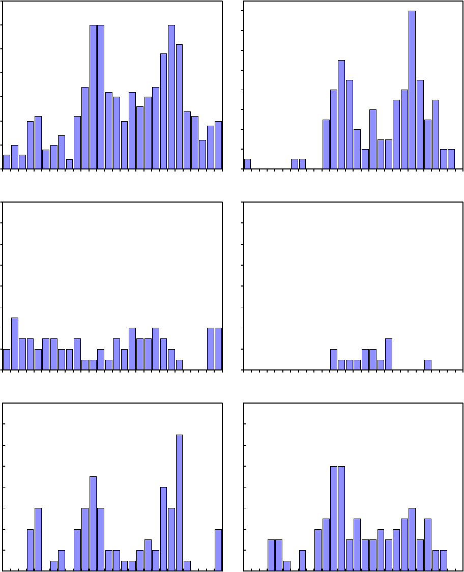
• They tend to cluster around certain years, such as 1974-75, 1982-83, 1991-93 and
1997-98 (Figure 1). This clearly points to the influence of some common external or
other causes, such as the oil shocks or the Asian crisis.
• They are generally quite severe. The severity of the recession is –8.7 percent on
average for the overall sample, and annual growth during a recession episode is on
average –6.5 percent relative to trend growth (Table 1). This represents a very large
fall in real GDP growth. In most cases, growth turns negative during a recession.
However, in a few cases, where trend growth is very high, growth may remain
positive while falling significantly below trend growth.
• They tend to be relatively short. The average length of a recession is 1.3 years,
reflecting the fact that 75 percent of the episodes are only one-year long while only a
few episodes are more than four-years long.
• There is a lot of variance among recession episodes. The standard deviation is thus
6.1 percent for the severity of a recession and 0.7 years for the length.
There are also important differences across country groups. Recessions are more severe on
average in the Middle East, Western Hemisphere and in countries in transition, and less
severe in advanced economies.
Table 1. Overview of Recessions
Area Number of episodes Depth Length Growth (relative to long term growth)
Before During After
AFR 84 -9.5 1.3 0.4 -7.3 1.0
ASIA 52 -8.0 1.3 0.3 -6.0 0.4
MED 13 -10.5 1.1 -0.8 -9.6 -0.4
ADV 61 -5.8 1.4 -0.6 -4.4 0.0
WHD 59 -10.3 1.5 0.3 -7.1 0.8
TRANS 7 -11.9 1.3 -3.8 -9.3 -0.3
ALL
276
-8.7
(6.1)
1.3
(0.7)
0.0
(3.2)
-6.5
(3.1)
0.5
(3.1)
Note: the table presents unweighted averages, standard deviations for the overall sample are in parentheses.
- 8 -
Figure 1. Number of Countries in Recessions, 1971-98
0
5
10
15
20
25
30
35
1971 1974 1977 1980 1983 1986 1989 1992 1995 1998
ALL
AFR
0
2
4
6
8
10
12
14
16
1971 1974 1977 1980 1983 1986 1989 1992 1995 1998
ASIA
0
2
4
6
8
10
12
14
16
1971 1974 1977 1980 1983 1986 1989 1992 1995 1998
ME
0
2
4
6
8
10
12
14
16
1971 1974 1977 1980 1983 1986 1989 1992 1995 1998
ADV
0
2
4
6
8
10
12
14
16
1971 1974 1977 1980 1983 1986 1989 1992 1995 1998
WH
0
2
4
6
8
10
12
14
16
1971 1974 1977 1980 1983 1986 1989 1992 1995 1998

- 9 -
B. Fiscal Response During a Recession
On average, the fiscal response during a recession is expansionary (Table 2). There are,
however, differences between country groups: advanced economies exhibit by far the largest
expansionary fiscal response (about -3 percent of GDP on average), while Middle East and
Western Hemisphere countries have on average a slightly contractionary fiscal response. To
examine the effectiveness of fiscal policy, recession episodes are then divided into two
groups, those where fiscal policy was expansionary and those where it was contractionary.
Table 2. Fiscal Policy During Recession Episodes
Area Number of episodes Fiscal response Fiscal deficit
Before During After
AFR 84 -1.1 4.8 5.4 5.3
ASIA 52 -0.9 4.5 5.2 4.7
MED 13 0.2 5.6 4.7 4.5
ADV 61 -3.1 1.3 3.2 3.5
WHD 59 0.5 4.0 4.1 2.9
TRANS 7 -0.5 6.0 6.2 4.0
ALL
276
-1.1
(5.6)
3.9
(4.7)
4.6
(4.1)
4.2
(4.2)
Note: the table presents unweighted averages, standard deviations for the overall sample are in parentheses.
Fiscal policy appears procyclical in 40 percent of the recession episodes (Table 3).
10
The two
groups are clearly differentiated, with a fiscal response of about –3¾ percent of GDP for
expansionary episodes compared to +3 percent of GDP for contractionary episodes, even
though the variance around these numbers is quite large There are also interesting differences
between country groups: in particular, fiscal policy is more often expansionary and fiscal
contractions tend to be smaller in advanced economies than in the other regions. This result is
consistent with, and generalizes, the findings of Gavin and Perotti (1997) that fiscal policy is
more countercyclical in advanced economies than in other regions (in their paper, the
comparison is with Latin America).
The stance of fiscal policy in a recession appears to be strongly correlated with the country’s
fiscal situation prior to the recession. The fiscal deficit prior to the recession is significantly
larger for episodes accompanied by a fiscal contraction than for episodes accompanied by a
fiscal expansion. This result holds for all the groups, with the difference being particularly
striking for advanced economies and Middle East countries. Public debt is also higher on
10
Due to the small size of the sample, results for countries in transition are not shown in the rest of the paper,
although they remain included in the overall sample.

- 10 -
average before contractionary episodes (Table 4). Government size, as measured by revenue-
to-GDP ratio, is larger for episodes with expansionary fiscal policy. Even though this result is
partly driven by advanced economies, it holds for most of the groups and may be explained
by the fact that automatic stabilizers are larger in countries with a large government.
Table 3. Expansionary versus Contractionary Fiscal Response During Recessions
Expansionary fiscal response
Area
Number of
episodes
Percent of total Fiscal response
Fiscal deficit
Before During After
AFR 49 58 -4.0 3.6 6.4 6.5
ASIA 26 50 -3.2 2.8 5.3 4.3
MED 7 54 -4.4 2.4 5.6 3.6
ADV 49 80 -4.1 0.3 2.8 3.1
WHD 30 51 -3.8 3.2 6.1 4.4
ALL
166
60
-3.8
(4.7)
2.5
(4.2)
5.1
(3.9)
4.6
(4.0)
Contractionary fiscal response
Area
Number of
episodes
Percent of total Fiscal response
Fiscal deficit
Before During After
AFR 35 42 3.0 6.4 4.1 3.6
ASIA 26 50 1.5 6.2 5.0 5.2
MED 6 46 5.5 9.3 3.8 5.5
ADV 12 20 0.8 5.4 4.6 5.1
WHD 29 49 4.9 4.9 2.0 1.3
ALL
110
40
3.0
(4.4)
6.0
(4.6)
3.7
(4.3)
3.6
(4.3)
Note: the table presents unweighted averages, standard deviations for the overall sample are in parentheses.
Fiscal policy during a recession also appears strongly linked to external factors. In particular,
expansionary episodes are accompanied on average by a deterioration in the terms of trade,
while episodes with a contractionary fiscal response are characterized on average by an
improvement in the terms of trade. This result applies to all the country groups. One possible
explanation is that terms of trade shocks directly affect the fiscal deficit in many countries
(e.g. through export duties). A deterioration in the terms of trade would thus both increase the
fiscal deficit and reduce growth. Another possible explanation is that governments are more
prone to let the deficit increase when the recession is caused by a negative terms of trade
shock than when it is caused by other factors. The current account deficit is also generally

- 11 -
larger before episodes accompanied by a contractionary fiscal response, which could reflect
the impact of external financing constraints.
Finally, recessions accompanied by a contractionary fiscal response are also characterized by
higher inflation. This may be explained by the fact that a number of recession episodes in
these regions are in countries with very high rates of inflation, and contractionary fiscal
policy is only one element of a broader stabilization package.
Table 4. Factors Related to the Stance of the Fiscal Response
Expansionary fiscal response
Area Public debt Government size Terms of trade Current account balance Inflation
Number of
episodes
In percent
of GDP
Number of
episodes
Revenue
to GDP
Number of
episodes
In percent
of GDP
Number of
episodes
In percent
of GDP
Number of
episodes
In
percent
AFR 48 66.5 49 24.8 49 -3.0 43 -4.8 48 13.7
ASIA 20 23.4 26 24.7 24 -1.9 23 -2.4 25 6.7
MED 6 12.1 7 30.1 7 -13.9 6 0.6 7 17.7
ADV 47 24.2 49 39.8 44 -2.1 46 -2.3 49 10.3
WH 27 31.2 30 23.1 30 -0.1 28 -4.2 24 19.5
ALL 153 38.4 166 29.3 159 -2.6 151 -3.4 156 12.7
Contractionary fiscal response
Area Public debt Fiscal size Terms of trade Current account balance Inflation
Number of
episodes
In percent
of GDP
Number of
episodes
Revenue
to GDP
Number of
episodes
In
percent
Number of
episodes
In percent
of GDP
Number of
episodes
In
percent
AFR 34 47.9 35 21.3 35 5.7 34 -5.3 35 16.0
ASIA 20 27.1 26 21.2 26 2.6 26 -2.0 26 11.8
ME 6 47.8 6 29.6 6 9.2 6 -3.9 5 15.5
ADV 11 55.9 12 35.4 11 4.0 12 -1.2 12 7.1
WH 24 35.5 29 21.5 29 3.8 27 -5.6 23 21.0
ALL 97 40.9 110 23.6 109 4.6 107 -4.1 101 15.0
Turning to the composition of fiscal policy, expansionary fiscal responses generally reflect
increases in public expenditure rather than tax cuts, while contractionary responses are
achieved through a mix of tax increases and expenditure cuts (Table 5). The asymmetry of
expansionary fiscal responses is particularly striking for Africa, advanced economies and
Western Hemisphere countries, and is observed in all country groups except Middle East. It

- 12 -
is also interesting to note that advanced economies are the only group in which expenditures
increase even when the fiscal response is contractionary.
Table 5. Composition of Fiscal Response During a Recession
Expansionary fiscal response
Area Number of episodes Change in expenditure Change in revenue
AFR 49 2.2 -0.6
ASIA 26 1.5 -1.0
ME 7 -0.1 -3.3
ADV 49 2.8 0.3
WH 30 2.9 0.1
ALL 166 2.2 -0.4
Contractionary fiscal response
Area Number of episodes Change in expenditure Change in revenue
AFR 35 -1.2 1.1
ASIA 26 -1.3 0.0
ME 6 -3.3 2.3
ADV 12 1.6 2.4
WH 28 -1.9 1.1
ALL 109 -1.2 1.0
C. Fiscal Response and Economic Activity in a Recession
On average, recession episodes accompanied by an expansionary fiscal response are less
severe. The average severity of recessions accompanied by an expansionary fiscal response is
–8.4 percent, compared to –9.2 percent for episodes characterized by a contractionary fiscal
policy (Table 6). The difference is largest in Asian and Western Hemisphere countries, and
holds for all country groups except Africa and advanced economies. On an annual basis (i.e.
abstracting from differences in the length of recession), all country groups have higher
growth relative to trend during episodes with expansionary fiscal policy compared to those
with contractionary fiscal policy. Endogeneity of the fiscal response would lead to the
opposite correlation.
On the other hand, growth immediately after the recession is not systematically higher or
lower depending on the stance of fiscal policy during the episode. However, as recessions
- 13 -
accompanied by contractionary fiscal policy are generally deeper, the rebound in growth
tends to be larger after contractionary fiscal responses.
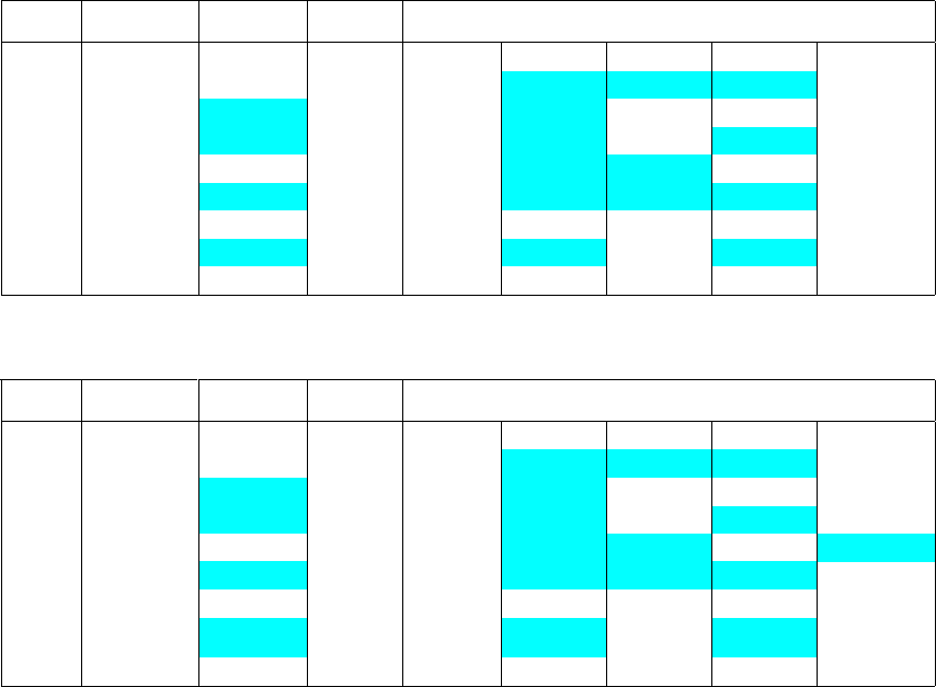
Table 6. Growth and Fiscal Response During Recession Episodes
Expansionary fiscal response
Area
Number of
episodes Severity Length Growth (relative to trend growth)
Before During After Decline Rebound
AFR 49 -9.9 1.4 0.1 -7.1 1.1 -7.3 8.2
ASIA 26 -7.6 1.2 0.4 -6.0 0.2 -6.3 6.2
MED 7 -10.3 1.1 -2.4 -8.6 -1.1 -6.2 7.5
ADV 49 -5.9 1.4 -0.4 -4.3 0.0 -3.9 4.4
WHD 30 -9.5 1.4 0.4 -6.8 0.8 -7.2 7.6
ALL 166 -8.4 (6.1) 1.4 (0.6) 0.0 (2.6) -6.2 (3.0) 0.5 (3.1) -6.1 6.6
Contractionary fiscal response
Area
Number of
episodes Severity Length Growth (relative to trend growth)
Before During After Decline Rebound
AFR 35 -9.0 1.2 0.7 -7.7 1.0 -8.4 8.6
ASIA 26 -8.3 1.3 0.2 -6.0 0.6 -6.2 6.6
MED 6 -10.7 1.0 1.1 -10.7 0.6 -11.8 11.2
ADV 12 -5.5 1.2 -1.2 -4.5 -0.3 -3.4 4.3
WHD 29 -11.2 1.6 0.2 -7.4 0.8 -7.5 8.2
ALL
110
-9.2
(6.1)
1.3
(0.7)
0.0
(3.9)
-7.1
(3.1)
0.7
(3.1)
-7.1
7.7
Shaded areas indicate observations consistent with effective fiscal policy as defined in Section II
To examine the influence of various factors on the relationship between fiscal policy and
growth during a recession, the sample is further split based on the values taken by both the
fiscal response and each of the relevant factors. Three broad categories of factors are
distinguished: (i) initial conditions, (ii) the composition of fiscal policy, and (iii)
accompanying policies.
Initial conditions
Openness and exchange rate regime
In principle, the effectiveness of fiscal policy in stimulating economic activity depends on
whether an economy is open or not, and on the exchange rate regime and degree of capital
mobility. Fiscal policy is less effective in open economies than in closed economies because

- 14 -
there is some crowding out through imports. With capital mobility, the effectiveness of fiscal
policy in an open economy is further reduced with a flexible exchange rate, while it is
increased (and possibly more than in a closed economy) with a fixed exchange rate. In the
absence of data on the degree of capital mobility, the analysis here distinguishes between
only three categories: closed economy, open economy with a flexible exchange rate, and
open economy with a fixed exchange rate.
Expansionary fiscal policy is associated with less severe recessions in closed economies or in
open economies with a fixed exchange rate (Table 7). Contractionary fiscal policy is then
associated with more severe recessions than in open economies with a flexible exchange rate.
These results appear remarkably consistent with the predictions of theory (assuming some
capital mobility).
Table 7. Openness and Exchange Rate Regime
Growth during recession Fiscal Policy
Expansionary Contractionary All
-5.8 -7.6 -6.6
-7.1 -6.3 -6.7
Closed
Open, and flexible exchange rate
Open, and fixed exchange rate
-6.1 -7.0 -6.4
Number of episodes: 118. Openness is defined as imports-to-GDP ratio higher than 30 percent.
Fiscal conditions
When initial fiscal conditions are favorable, expansionary fiscal policy appears to be
more effective. In particular, when public debt is relatively low before a recession (below 50
percent of GDP), expansionary fiscal responses are associated with better growth outcomes
during the recession than contractionary responses, whereas when public debt is high, the
fiscal stance appears to make no difference for the severity of the recession (Table 8). This is
consistent with the theoretical prediction that fiscal policy is less effective and crowding out
larger when public debt is high. On the other hand, the level of the fiscal deficit before a
recession does not seem related to the effectiveness of fiscal policy, whereas it appeared
important in determining the choice of the fiscal response, as shown in Table 3. One
interpretation is that it may be difficult to finance an increase in an already large deficit, but a
large deficit does not in itself necessarily signal sustainability problems, and may therefore
not reduce the effectiveness of fiscal policy. Moreover, fiscal policy appears to be more
effective in countries with a large government.

- 15 -
Table 8. Initial Fiscal Conditions and Fiscal Response
Growth during recession
Fiscal policy
Expansionary Contractionary All
High Yes
-6.9 -7.0 -6.9
public debt No
-6.0 -7.1 -6.4
before recession All
-6.2 -7.0 -6.5
Number of episodes: 250. High public debt is defined as higher than 50 percent of GDP
Growth during recession
Fiscal policy
Expansionary Contractionary All
Large Yes
-6.7 -7.2 -7.0
fiscal deficit No
-6.0 -6.8 -6.2
before recession All
-6.2 -7.1 -6.5
Number of episodes: 276 (full sample). Large fiscal deficit is larger than 5 percent of GDP.
Growth during recession
Fiscal policy
Expansionary Contractionary All
Large Yes
-4.8 -6.2 -5.2
government size No
-7.2 -7.4 -7.3
before recession All
-6.2 -7.1 -6.5
Number of episodes: 276 (full sample). Large government is when revenue-to-GDP is higher than 30 percent.
External conditions
Similarly, a sound external position before the recession leads to expansionary fiscal
response being accompanied by higher growth. Conversely, when the current account deficit
is large before the recession (i.e. above 5 percent of GDP), contractionary fiscal responses
are associated with higher growth (Table 9).
Table 9. Current Account Deficit Before Recession and Fiscal Response
Growth during recession
Fiscal policy
Expansionary Contractionary All
Large Yes
-7.6 -7.2 -7.4
current account deficit No
-5.6 -6.9 -6.1
before recession All
-6.2 -7.0 -6.6
Number of episodes: 258
Composition of fiscal policy
Expansionary fiscal policy appears to be more effective when it is expenditure-led during a
recession. On the other hand, there is virtually no difference for contractionary fiscal
responses (Table 10).

- 16 -
Table 10. Composition of Fiscal Policy and Fiscal Response
Growth during recession
Fiscal policy
Expansionary Contractionary All
Expenditure-led Yes
-5.8 -7.2 -6.3
Fiscal response No
-6.9 -7.0 -6.9
All
-6.2 -7.1 -6.5
Number of episodes: 275
Accompanying policies
Monetary policy
Fiscal policy appears to be more expansionary when monetary policy is also expansionary,
with an average increase in interest rates of 0.7 percent versus 1.2 percent. This makes it
difficult to disentangle the effects of monetary and fiscal policy in a recession. But, on
average, a recession is more severe when both monetary and fiscal policy are contractionary
than when they are both expansionary
11
(Table 11). These results are in line with the
predictions of the theory. Conversely, when monetary policy is restrictive, fiscal policy does
not seem to make much of a difference.
Table 11. Policy Mix and Growth During Recession Episodes
Growth during recession
Fiscal policy
Expansionary Contractionary All
Expansionary
-5.0 -5.6 -5.2
Monetary policy Contractionary
-6.5 -6.7 -6.6
All
-5.9 -6.3 -6.1
Number of episodes: 171
Exchange rate policy
Recessions preceded by an exchange rate depreciation are more severe on average than
recessions preceded by an appreciation, and their severity does not appear to be related to the
fiscal response. Similarly, exchange rate policy during a recession does not modify the
effectiveness of fiscal policy except that contractionary fiscal policy appears less costly when
accompanied by an exchange rate depreciation (Table 12).
11
Similar results are obtained when using the change in M2 to GDP.

- 17 -
Table 12. Exchange Rate Policy Before and During Episodes
Growth during recession
Fiscal Policy
Expansionary Contractionary All
Exchange rate Yes
-7.0 -6.9 -7.0
depreciation No
-4.7 -6.8 -5.4
before recession All
-6.2 -6.9 -6.5
Number of episodes: 229
Growth during recession
Fiscal Policy
Expansionary Contractionary All
Exchange rate Yes
-6.4 -6.9 -6.6
depreciation No
-5.6 -7.5 -6.3
during recession All
-6.2 -7.1 -6.5
Number of episodes: 276
D. Sensitivity Analysis
This section examines the sensitivity of the results to changes in the sample and to the
definitions used.
Sample
The results presented above are based on a sample in which outliers—defined as episodes
with growth or an overall balance to GDP above 15 percent in absolute terms—were
excluded. Since this criterion is arbitrary, we need to check how it may influence the results.
Alternative criteria for outliers, such as a cut off value of 10 percent rather than 15 percent,
or the exclusion of the extreme quintiles or deciles were thus explored. Table 13 shows that
even though the sample size varies substantially, the results are not very different.
Table 13. Impact of Filtering Method on Sample Size and Results
Filtering method Number of episodes Impact of fiscal response on growth (1)
+/-15 percent interval 276 0.9
+/-10 percent interval 199 0.7
1st and last quintiles excluded 216 0.7
1st and last deciles excluded 124 0.8
(1) Difference between average growth during episodes with expansionary and contractionary fiscal response
Selection bias
Another possible bias comes from the criterion used to define recessions. As growth during a
recession is measured by the difference between actual and trend growth, it is by definition
bounded by the standard deviation of real GDP growth for the country. This could result in

- 18 -
an undesired correlation between our measure of growth during a recession and the standard
deviation (which can be seen as a proxy for the volatility of real GDP growth) if growth
during was always very constrained by its upper bound. The average difference between
growth during a recession and this bound is 3.2 percent for the overall sample. It therefore
appears large enough—as a comparison, the standard deviation of real GDP growth is 4.4
over the sample—to suggest the definition of recession episodes does not bias the results.
12
E. Preliminary Findings
Overall, many of the observations in this section appear to be broadly in line with theoretical
predictions and the following stylized facts emerge:
• On average, fiscal policy is expansionary during recession episodes. However, a very
large number of recession episodes (40 percent of total) are accompanied by
contractionary fiscal policy. Unfavorable initial conditions (high public debt, and
large fiscal and current account deficits) are associated with a contractionary fiscal
response in a recession, while negative terms of trade shocks or a large public sector
tend to result in a more expansionary fiscal response.
• There is some evidence that expansionary fiscal policy dampens the severity of a
recession, especially in open economies with a fixed exchange rate, favorable initial
fiscal and external conditions (low public debt, a large public sector, and a small
current account deficit), and in combination with expansionary monetary policy.
Expenditure-led fiscal expansions are also associated with less severe recessions. All
these results are consistent with the predictions of the theory, even though the
magnitude of the average effects is small, and the variance is large.
• There are marked differences between advanced economies and other country groups.
The fiscal response is more often expansionary in advanced economies. At the same
time, the impact of fiscal policy tends to be smaller than in other groups.
• A number of other factors are associated with both the fiscal response and the severity
of a recession. Inflation tends to be higher, and monetary policy more contractionary
during episodes with a contractionary fiscal response, which makes the interpretation
of the results somewhat difficult and points to the need for a multivariate approach.
However, the methodology used here does not allow strong inferences on the relationships
between the different variables. In addition, the variance in the sample suggests that the
observed differences may not be significant. These issues will be examined in the regression
analysis presented in section V.
12
The result holds for each of the country group.

- 19 -
IV. E
XPLORATORY
M
ULTIDIMENSIONAL
A
NALYSIS
A. Rationale
The descriptive analysis of the previous section provides some insights into the nature and
impact of the fiscal response in a recession. However, it also suggests that many different
factors have to be taken into account simultaneously when assessing the relationship between
the main variables of interest. In this section a multidimensional analysis is used to identify
typologies of recession episodes and the associated fiscal responses. More specifically, the
idea is to identify episodes that constitute relatively homogenous groups for the variables of
interest and the key characteristics of these groups. The approach is exploratory since there
are no prior assumptions relating the variables. It is also multidimensional as it tries to
analyze the simultaneous interactions among these variables. To this end, two different
statistical techniques are used in sequence: principal components analysis and cluster
analysis.
Multidimensional statistical methods are designed to explain the correlations or covariances
among a set of variables in terms of a limited number of unobservable or latent variables
(Lebart, Morineau, and Piron, 1995). In reducing the number of original variables into a new
set of factors, these methods can extract information present in the original data that cannot
be observed directly either because it is difficult to measure (for instance, the set of initial
conditions discussed in the previous section) or because economic variables tend to be
measured with error. Principal components analysis is particularly useful in identifying a
small number of dominant factors among a large number of observed variables that explain
most of the variance of the original data (Dunteman, 1980). These factors or principal
components are linear combinations of the original variables, and can be interpreted on the
basis of their relation with the original variables.
13
Cluster analysis is then applied to the results of the principal components analysis to partition
the sample of recession episodes into homogenous groups. The objective is to sort episodes
into groups so that the degree of statistical association is high among members of the same
group and low between members of different groups (Everitt, 1974). Since it does not require
any assumption on the distribution of the variables in the population, the method is widely
used as an exploratory data analysis tool (Diday, 1982). However, since cluster analysis is a
descriptive rather than a probabilistic statistical method, it cannot be used to test any
hypothesis concerning the causal relationship between variables (Morrison, 1980). The
advantage of carrying out cluster analysis on the principal components is that groups can be
identified according to multidimensional concepts not directly observable in the original data.
13
For each factors, factor scores are calculated as a linear transformation of the standardized original variables
with weights proportional to the correlation coefficients between the original variables and the factor.

- 20 -
B. Principal Components Analysis
Principal components analysis aims at determining the coefficients that relate the observed
variables to a reduced number of dominant factors.
14
The key problems are how the
determine the optimal number of factors and how to interpret them. Two main criteria are
used. First, only factors that explain a larger portion of the total variance than individual
variables are extracted.
15
Second, these factors are interpreted, and hence labeled, by looking
at their correlation with the original variables. Principal components analysis is thus
performed on a matrix of 224 downturn episodes,
16
including the following groups of
variables identified in the previous section:
• nature of the recession (average growth during the episode and its length);
• fiscal response and composition of fiscal adjustment;
• initial conditions (fiscal deficit, debt, current account deficit, openness, etc..);
• accompanying monetary and exchange rate policies.
Eight principal components are identified, explaining about 75 percent of the total variance,
and the remaining 25 percent can be seen as a residual not related to the common
characteristics of the data. The factors are reported in Table 14 for each principal component
and can be interpreted as follows.
• Size of government. The first principal component is positively correlated with high
ratios of expenditure and revenue to GDP.
• Fiscal response. The second factor is correlated with fiscal responses and increases
in public expenditure, combined with small initial fiscal deficits (or fiscal surpluses).
• Terms of trade change during episode. The third principal component is strongly
and positively correlated with terms of trade improvements during the recession.
• Openness and financial depth along with monetary policy response. The fourth
factor is positively correlated to openness, expansionary monetary policy and
financial depth, as measured by the ratio of M2 to GDP.
14
These coefficients are called factor loadings and can be seen as playing a role similar to coefficients in
standard multivariate regression analysis.
15
In mathematical terms, this means that only factors with eigenvalues higher than one have been retained. To
identify principal components, we use Kaiser’s varimax criterion to orthogonally transform the original data.
16
The number of recession episodes is reduced from 276 to 224 when all the variables of interest are included in
the sample.
- 21 -
Table 14. Rotated Components Matrix and Total Variance Explained
• Initial conditions (public debt, reserves ratio and current account deficit). The fifth
factor is negatively correlated to favorable initial conditions;
• Macroeconomic conditions before the episode (inflation and growth before the
episode). The sixth component is positively correlated with low levels of inflation and
relatively high growth before the recession episode;
• Change in revenues. The seventh component is positively correlated with an
increase in the revenue-to-GDP ratio; and
• Change in the exchange rate. The final factor is positively correlated with the
change in depreciation during the recession.
Variables Components
12345678
Expenditures to GDP, before
0.93
-0.08 -0.01 0.17 -0.08 -0.11 -0.04 0.04
Revenues to GDP, before
0.91
0.20 -0.03 0.22 0.05 -0.10 -0.06 0.03
Growth during 0.57 0.05 0.04 -0.36 0.27 0.32 0.12 -0.19
Fiscal response -0.05
-0.93
0.13 -0.04 -0.01 -0.07 0.11 -0.01
Fiscal balance before 0.07
0.77
-0.04 0.17 0.33 -0.02 -0.06 -0.01
Change in expenditure to GDP 0.01
0.69
-0.09 0.03 0.01 0.05 0.68 0.00
Terms of trade shock -0.02 -0.09
0.99
0.00 -0.02 0.00 0.00 -0.01
Openess, before 0.21 0.13 0.08
0.79
-0.15 -0.09 -0.09 -0.04
Monetary response -0.08 0.06 -0.04
0.65
0.13 0.41 0.12 -0.04
M2 to GDP before 0.41 0.07 -0.10
0.61
0.32 0.01 0.01 -0.08
Current account balance, before 0.18 0.12 -0.05 -0.03
0.71
0.11 0.03 -0.08
Public debt before 0.06 -0.03 -0.03 0.05
-0.70
0.11 -0.12 -0.11
Reserves to imports before -0.04 0.10 -0.03 0.20
0.55
-0.08 -0.26 0.08
Inflation before -0.04 -0.08 0.06 -0.11 0.03
-0.85
0.05 0.03
Growth before -0.11 -0.02 0.05 -0.03 -0.06
0.73
0.03 0.16
Change in revenues to GDP -0.04 -0.16 0.03 -0.01 0.00 -0.02
0.96
-0.01
Change in exchange rate -0.11 -0.05 0.07 0.03 -0.05 0.04 0.01
0.75
Length of recession 0.11 0.06 -0.09 -0.11 0.14 0.07 -0.02
0.73
Sums of squared loadings 2.31 2.09 2.04 1.73 1.66 1.59 1.52 1.20
Total variance explained
In percent of total variance 12.16 11.00 10.74 9.10 8.72 8.36 8.02 6.30
Cumulative 12.16 23.16 33.90 43.00 51.72 60.08 68.11 74.41
Extraction Method: Principal Component. Rotation Method: Varimax with Kaiser Normalization, converged in 8 iterations.

- 22 -
C. Cluster Analysis
The eight factors thus identified are then used as input variables in the cluster analysis.
Selecting the optimal number of clusters is to some extent a subjective exercise. Using
alternative clustering algorithms ensures that robust partitions of the sample are identified.
Nonetheless, smaller clusters may present difficulties because they may not be easily
assimilated to other clusters as they tend to capture outliers. The strategy adopted here is to
select a limited number of large clusters while grouping the remaining clusters and outliers
into a single composite group.
Using a non-hierarchical algorithm (see Appendix II),
17
seven clusters representing 202
episodes are identified, while the remaining 22 episodes are grouped in a residual cluster.
18
The distribution of episodes by cluster membership and region is presented in Table 15.
19
Advanced economies are concentrated in cluster 3, which groups 61 percent of the episodes
for this region. More than half of the Asian countries are in cluster 6. Middle Eastern
countries are mostly in cluster 7. Other regions tend to be more evenly spread across clusters,
although countries in transition are in a large part in clusters 3 and 8, African countries in 2
and 6, and Western Hemisphere countries in 1 and 6. Most of the 1998 Asian crisis countries
are included in cluster 7. Outliers (cluster 8) are fairly evenly distributed across regions,
except for an over-representation of countries in transition.
Descriptive statistics and tests are calculated within each cluster and across clusters to
identify variables that are significantly different from the sample average (Table 16).
20
Active
variables that are used in the principal components and cluster analysis are distinguished
from illustrative variables that are helpful in describing the characteristics of the clusters.
17
Appendix II briefly reviews cluster analysis and clustering algorithms. As changes in the pre-determined
number of clusters can produce groups with different characteristics, a robustness check using alternative
numbers of partitions was conducted. It showed that the identified clusters are relatively stable implying that
they identify “strong partitions” in the original data.
18
Caution is needed in the interpretation of the results for this cluster as it aggregates smaller clusters and
isolated episodes (outliers).
19
A list of all episodes by clusters is reported in Table A2 in Appendix II.
20
Non parametric statistics are also used to test the assumption that the means are equal across the groups and
confirm they are statistically different across the clusters.

- 23 -
Table 15. Clusters Composition by Region
Four clusters (47 percent of the sample) group countries that responded to the recession with
expansionary fiscal policies.
• Cluster 1 (29 episodes) groups episodes with the most severe recessions, both in
terms of the average growth and the length of the recession. African and Western
Hemisphere countries account for 80 percent of the episodes in this cluster. The fiscal
policy is driven by higher spending while monetary policy is restrictive. Government
size tends to be small and financial sectors not particularly developed. In addition, the
episodes are accompanied on average by large negative terms of trade shocks and
exchange rate depreciations—especially the three Argentina episodes (1981-82, 1985,
and 1989), Costa Rica (1980-82), Mexico (1982-83), and Sierra Leone (1991-92)—
preceded by relatively high inflation rates.
• Cluster 2 (29 episodes) contains relatively short recessions of average depth. Fiscal
expansion is sizeable (about 4½ percent of GDP), driven by a mix of expenditure
increases and, to a lesser extent, tax cuts, and accompanied by a mild monetary
contraction. Initial conditions point to a mix of high public debt—the Gambia (1994),
Madagascar (1991), Tanzania (1992), and Jamaica (1988)—and large current account
deficits—Chile (1982-85), Honduras (1982-83), Madagascar (1991), and Nigeria
(1987). Inflation is relatively low both before and during the recession. Similar to the
Area Clusters12345678Total
ADV No. 12311751351
in percent of area 2.0 3.9 60.8 2.0 13.7 9.8 2.0 5.9 100.0
in percent of cluster 3.4 6.9 79.5 6.7 25.9 9.3 11.1 13.6 22.8
AFR No.
12 16 2 8 9 18 1 9 75
in percent of area 16.0 21.3 2.7 10.7 12.0 24.0 1.3 12.0 100.0
in percent of cluster 41.4 55.2 5.1 53.3 33.3 33.3 11.1 40.9 33.5
ASIA No. 41224193136
in percent of area 11.1 2.8 5.6 5.6 11.1 52.8 8.3 2.8 100.0
in percent of cluster 13.8 3.4 5.1 13.3 14.8 35.2 33.3 4.5 16.1
MED No. 12418
in percent of area 12.5 25.0 50.0 12.5 100.0
in percent of cluster 3.7 3.7 44.4 4.5 3.6
TRANS No.
112 1 27
in percent of area 14.3 14.3 28.6 14.3 28.6 100.0
in percent of cluster 3.4 3.4 5.1 3.7 9.1 3.1
WHD No. 11924510 647
in percent of area 23.4 19.1 4.3 8.5 10.6 21.3 12.8 100.0
in percent of cluster 37.9 31.0 5.1 26.7 18.5 18.5 27.3 21.0
Total No. 29 29 39 15 27 54 9 22 224
in percent of area 12.9 12.9 17.4 6.7 12.1 24.1 4.0 9.8 100.0
in percent of cluster 100.0 100.0 100.0 100.0 100.0 100.0 100.0 100.0 100.0

- 24 -
Table 16. T-tests and Kruskal-Wallis Tests by Variables and Clusters
Clusters Cluster no. 1 Cluster no. 2 Cluster no. 3 Cluster no. 4 Cluster no. 5 Cluster no. 6 Cluster no.7 Cluster no. 8 Total
Active variables Mean t-test Mean t-test Mean t-test Mean t-test Mean t-test Mean t-test Mean t-test Mean t-test Mean K-W Median
Growth
Growth during -8.2 *** -6.7 -3.8 *** -8.9 *** -5.7 -5.8 ** -8.9 -8.1 ** -6.4 *** ***
Length of recession 1.6 1.1 *** 1.6 ** 1.1 *** 1.3 1.1 *** 1.1 * 1.8 1.3 *** ***
Growth before 0.2 0.1 -0.1 0.3 -1.3 ** 1.2 ** -1.7 ** -1.9 -0.1 **
Policy response
Fiscal response -1.1 -4.3 *** -2.2 *** 1.0 ** 2.9 *** 0.3 *** -2.3 * -0.8 -0.8 *** ***
Monetary response -0.5 *** 0.5 0.8 -0.1 ** 0.7 1.9 9.3 ** 3.6 1.4 *** **
Initial conditions
Public debt before 35.1 54.2 ** 27.9 *** 52.8 ** 56.3 *** 31.1 *** 14.1 *** 52.6 40.0 *** ***
Fiscal balance before -5.0 * -0.7 *** -1.2 *** -7.6 -8.9 *** -4.8 -0.8 ** -3.7 -4.1 *** ***
Current account balance, bef. -5.0 -6.8 ** -1.7 *** -8.4 -5.3 -3.0 *** -1.8 -6.1 -4.4 *** ***
M2 to GDP before 29.0 *** 29.7 *** 56.5 *** 26.8 *** 41.9 34.0 *** 84.5 *** 46.9 40.5 *** ***
Inflation before 53.7 12.6 *** 9.3 *** 35.9 14.9 *** 26.3 ** 3.2 *** 281.2 48.5 ** **
Reserves to imports before 23.3 17.9 ** 20.0 14.8 *** 13.2 *** 22.2 69.6 ** 33.2 22.8 **
Revenues to GDP, before 16.3 *** 26.1 42.7 *** 22.9 31.6 ** 17.8 *** 33.6 ** 28.9 26.7 *** ***
Expenditures to GDP, before 21.3 *** 26.9 ** 43.9 *** 30.5 *** 40.4 *** 22.6 *** 34.4 32.5 30.8 *** ***
Composition of fiscal policy
Change in expenditures to GDP 1.2 2.6 *** 2.0 *** 0.1 * -2.6 *** 0.4 1.2 2.6 0.9 *** ***
Change in revenues to GDP 0.1 -1.6 *** -0.3 1.1 0.3 0.7 ** -1.1 1.7 0.2 *** ***
Other factors
Openness 40.3 35.9 33.3 24.0 *** 42.4 * 24.0 *** 60.1 *** 51.3 *** 34.9 *** ***
Exchange rate depreciation 240.6 *** 17.2 *** 10.9 *** 47.5 ** 65.4 *** 30.9 *** 14.8 *** 13830.8 1412.8 ** **
Terms of trade change -0.2 *** 0.0 0.0 0.3 *** 0.0 0.0 ** -0.1 0.1 0.0 *** ***
Cluster no. 1 Cluster no. 2 Cluster no. 3 Cluster no. 4 Cluster no. 5 Cluster no. 6 Cluster no.7 Cluster no. 8 Total
Descriptive variables Mean t-test Mean t-test Mean t-test Mean t-test Mean t-test Mean t-test Mean t-test Mean t-test Mean K-W Median
Depth of recession -12.45 *** -7.94 -6.31 *** -9.54 -7.50 -6.37 *** -10.2 -13.5 ** -8.55 *** ***
Growth after 0.74 *** 0.83 *** -0.43 *** 0.15 * 0.63 *** 1.12 *** -2.0 ** 0.4 0.44 *
Decline in growth -8.44 ** -6.81 -3.76 *** -9.14 ** -4.48 *** -6.98 -7.0 -6.2 -6.36 *** ***
Rebound in growth 8.98 ** 7.53 3.41 *** 9.02 * 6.36 6.95 6.8 8.5 6.89 *** ***
Change in interest rates 2.59 *** 1.18 -2.55 ** -0.80 -0.63 -0.11 0.3 0.7 -0.18 *** ***
Fiscal balance -6.13 *** -5.01 *** -3.42 *** -6.63 *** -5.92 *** -4.48 *** -3.1 *** -4.5 *** -4.84 ** *
Fiscal balance after -5.14 -5.15 -4.14 -4.89 -4.98 -4.44 -2.5 -3.7 -4.51
Inflation during 158.49 15.09 *** 11.03 *** 53.19 36.18 * 36.43 ** -2.2 ** 365.4 77.15 *** ***
Exchange rate depreciation, bef. -84.71 -94.98 -101.39 *** -84.46 -91.37 -93.09 -93.7 -81.0 -91.74 *** ***
T-test to verify that for each variable cluster means are equal to the sample means. KW test and median test are non parametric tests of the hypothesis that variable means are equal across clusters.
The tests' significance levels are denoted as a ten (*), five (**), and one (***) percent, respectively.
- 25 -
previous cluster, African and Western Hemisphere countries account for more than 80
percent of the episodes, with more than half of the episodes falling in the African
region.
• Cluster 3 (39 episodes) has relatively longer but milder recessions than the sample
average. Fiscal expansion is driven by expenditure increases and accompanied by
monetary expansion. Countries in this cluster are characterized by large government
sector and favorable initial conditions (e.g., low inflation, almost balanced current
account, and low public debt and fiscal deficit ratios to GDP). The bulk of the
episodes (85 percent) is in advanced economies, including Israel (1989). Exceptions
include South Africa (1990-92), Tanzania (1982-84), Barbados (1981-82 and 1990-
92), and Samoa (1990), and two countries in transition, Czech Republic (1998) and
Romania (1997-98).
• Cluster 7 (9 episodes) is similar to cluster 3, except for a more accentuated
expansionary monetary policy response and a more balanced fiscal response. Asian
and Middle Eastern countries account for most of the group. Although rather small,
this cluster is of particular interest since it features some of the Asian crises.
Recessions are on average shorter and deeper, and they occur against generally
favorable fiscal and external initial conditions, although macroeconomic conditions
are less so.
Three clusters, covering 43 percent of the sample, are characterized by contractionary fiscal
policy.
• Cluster 4 (15 episodes) groups recessions that are shorter than the sample average
but show a deeper decline in output. The fiscal contraction is relatively mild (one
percent reduction in the deficit), largely driven by higher revenue. Monetary policy
was also tightened. Initial fiscal conditions are rather unfavorable, particularly in the
case of Zambia (1994) and Honduras (1994). The same applies to initial external
conditions, with fairly large current account deficits in Madagascar (1981), Rwanda
(1991), and Samoa (1974). Countries in this cluster tend to be African (53 percent)
and Western Hemisphere countries (27 percent).
• Cluster 5 (27 episodes) contains episodes in which the fiscal contraction is more
accentuated than in the previous group and mostly driven by expenditure reduction.
The monetary response is moderately expansionary. Initial fiscal conditions are less
favorable than the sample average in terms of higher fiscal deficit prior to the crisis—
Cameroon (1988), Cote d’Ivoire (1983-82), and Tonga (1988)—and high public debt
ratios—Ethiopia (1991-92) and Togo (1983). Countries in this group are also
characterized by a large public sector and consist of advanced (26 percent) and
African (33 percent) economies. Advanced economies are represented by Belgium

- 26 -
(1983 and 1993) and Italy (1982 and 1993), two of the tales of expansionary fiscal
contractions discussed in Alesina and Ardagna (1998).
21
• Cluster 6 (54 episodes) is the largest and most robust group. These recession
episodes are relatively short and mild. Fiscal contraction is mild (0.3 percent of
GDP), pursued by a mix of revenue increase and expenditure reduction, and
accompanied by a moderate expansionary monetary policy (1.9 percent). Countries in
this group have on average a small public sector size and relatively favorable initial
conditions, both fiscal and non-fiscal. Asian and African countries account for 69
percent of the episodes in this cluster. Notable exceptions are Turkey (1989 and
1994), the United States (1980, 1982, 1991), and Japan (1974).
• Finally, cluster 8 (22 episodes or 10 percent of the sample) groups episodes
characterized by hyperinflation and consequent sharp devaluation—Brazil (1990),
Peru (1988-90), Belarus (1995) and Kazakhstan (1995)—countries with an unusually
high degree of openness—Hong Kong SAR and Singapore— and episodes with very
unbalanced initial fiscal and external positions—the Republic of Congo (1994),
Equatorial Guinea (1991), the Republic of Mozambique (1992) and Sudan (1983-84).
It also includes very long episodes, reaching to 6 years in the case of Trinidad and
Tobago (1983-89). Table 17 summarizes the main characteristics of each cluster.
In general, recession episodes for the same country tend to fall consistently within the same
cluster. This seems to reflect both the relative stability of key structural characteristics, such
as government size, and some persistence in policy responses to a crisis. However, a few
exceptions are worth noting. At one extreme we find the three Philippines episodes (1984,
1991, and 1998) falling in three different clusters—clusters 1, 6, and 4, respectively. The
different policy responses in the case of the Philippines may be dictated, among other things,
by a steady increase in the government size, from 12 percent in 1974 to 20 percent in 1998.
Other cases are the United States—with the 1980, 1982, and 1991 recession episodes
characterized by a contractionary response, whereas the earlier 1974 episode followed what
appears to be a standard advanced economy response (fiscal expansion driven by expenditure
increases and accompanied by accommodating monetary policy)—and India, with four
episodes—1972, 1976, 1979, and 1991—characterized by an overall contractionary response
vis-à-vis the expansionary fiscal policy pursued during the 1974 episode.
21
Two other well documented cases of expansionary fiscal contractions, namely Denmark (1983-86) and
Ireland (1987-89), discussed in Giavazzi and Pagano (1990) and reviewed in Hemming, Kell, and Mahfouz
(2000) are not captured by our definition of recession. This is not surprising since these are episodes of
sucessful fiscal contraction, characterized by high growth.

- 27 -
Table 17. Summary Qualitative Description of Clusters
Cluster 1 Cluster 2 Cluster 3 Cluster 4 Cluster 5 Cluster 6 Cluster 7
Growth
Growth during
Low
Average
High Low
Average
High
Low
Length of
recession
Long
Short Long Short
Average
Short
Short
Depth of
recession
Severe
Average
Mild
Severe Average
Mild
Severe
Policy response
Fiscal response Expan. Expan. Expan.
Contr. Contr. Contr.
Expan.
Monetary
response
Contr. Expan. Expan.
Contr.
Expan. Expan.
Expan.
Initial conditions
Public debt Average
High Low High High Low Low
Fiscal deficit Average
Small Small
Large
Large
Average
Small
Current account
deficit
Average
Large Small
Large Average
Small
Small
Inflation Average
Low Low
Average
Low Low Low
Fiscal size
Small
Average
Large
Average
Large Small
Average
Growth Average Average Average Average
Negative Positive Negative
Composition of
fiscal policy
Spending
Mix Spending
Revenue
Spending
Revenue Mix
Other factors
Terms of trade
Neg.
Average Average Positive Average Average Average
Exchange rate
dep.
Large Small Small Small
Average Small
Small
Inflation during High
Low Low
Average Low
Low Low
Region(s)
WHD
AFR
AFR
WHD
ADV
TRANS
AFR
WHD
AFR
ADV
ASIA
AFR
MED
ASIA
Bold characters identify variables that are different from the sample mean at a five percent significance level.
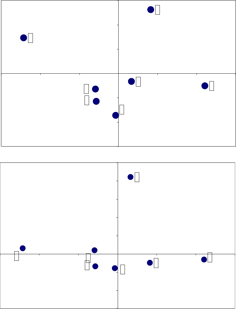
So far, clusters have been described on the basis of the within-cluster averages of each
variable. But the above described characteristics as well as differences and similarities
among the clusters can also be visually summarized by plotting all the cluster averages (or
centers) against selected principal components (Figures 2 and 3).
22
The following
observations can be highlighted, bearing in mind that these are purely illustrative.
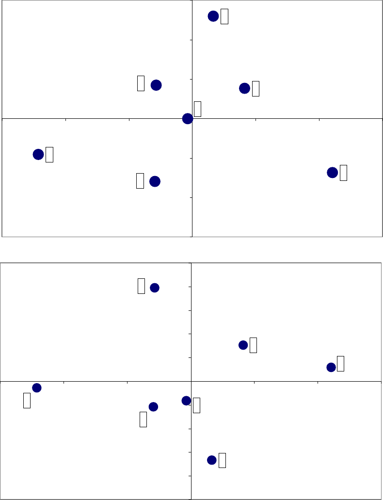
Clusters 1, 5, and 7 tend to lie in opposite portions of the charts. Cluster 1 clearly seems to
identify episodes characterized by expansionary fiscal responses with relatively unfavorable
initial fiscal and external conditions but average initial macroeconomic conditions (Figure 2,
22
These averages are calculated as averages of the factor scores for each principal components.
- 28 -
Figure 2. Distribution of Cluster Centers by Selected Factors
Fiscal response with initial fiscal, external and macroeconomic conditions
1/ Factor correlated with episodes showing fiscal response led by expenditure increases with favorable initial
fiscal balance
6
2
1
5
4
7
3
-1.5
-1.0
-0.5
0.0
0.5
1.0
1.5
-1.5 -1.0 -0.5 0.0 0.5 1.0 1.5
Fiscal response 1/
1
3
6
5
2
4
7
-0.5
-0.4
-0.3
-0.2
-0.1
0.0
0.1
0.2
0.3
0.4
0.5
-1.5 -1.0 -0.5 0.0 0.5 1.0 1.5
Initial macro conditions
Fiscal response 1/
Initial fiscal and
external conditions
- 29 -
Figure 3. Distribution of Cluster Centers by Selected Factors
Fiscal response with government size and monetary policy response
1/ Factor correlated with episodes showing fiscal response led by expenditure increases with favorable initial
fiscal balance
6
2
1
5
4
7
3
-1.5
-1.0
-0.5
0.0
0.5
1.0
1.5
-1.5 -1.0 -0.5 0.0 0.5 1.0 1.5
Fiscal response 1/
7
4
2
5
6
3
1
-1.5
-1.0
-0.5
0.0
0.5
1.0
1.5
2.0
2.5
-1.5 -1.0 -0.5 0.0 0.5 1.0 1.5
Openness, financial depth,
and monetray response
Fiscal response 1/
Government size
- 30 -
top and bottom panels). While sharing similar initial conditions, cluster 5 pursues opposite
fiscal responses. These seem to be associated with the fact that cluster 5 has on average a
larger government size (Figure 3, top panel). While showing a moderate expansionary fiscal
response, cluster 7 appears to have more favorable initial fiscal and external conditions as
compared with the other two clusters (Figure 2, top panel) but relatively unfavorable initial
macroeconomic conditions (Figure 2, bottom panel). Further, it appears to feature a more
expansionary monetary policy. However, regardless of these differences these groups seems
to be equally unsuccessful at dampening the fall in output during a recession.
Clusters 3 and 6 pursue different fiscal policies, in spite of the fact that they tend to lie on
the same portions of the charts in terms of initial conditions and accompanying monetary
policies. However, government size is much smaller in cluster 3 than in cluster 6. The
different fiscal policy responses in these groups lead, however, to similar recessions.
Cluster 2 and cluster 4 are quite similar in a number of respects. They share similar initial
unfavorable macroeconomic conditions, whereas cluster 4 has slightly more favorable fiscal
and external conditions (Figure 2, top and bottom panels). Their government sizes are below
the sample average. The most notable difference is that the fiscal response is more
contractionary in cluster 2 than in cluster 4, quite the opposite of their monetary responses.
Nonetheless, recessions appears less severe in cluster 2.
D. What Have We Learned?
As expected, when initial conditions, fiscal response and accompanying policies are
simultaneously analyzed in a multidimensional framework, the link between fiscal policy and
growth appears less clear than in the previous section. Considering the various groups that
emerged from the analysis, a number of general observations can be made.
• As indicated by the findings of the previous sections, initial conditions—fiscal,
external, and macroeconomic—are important factors in determining the effectiveness
of fiscal policy. The analysis of this section qualifies those findings by showing that it
is a combination of these initial conditions, as emerged via principal components
analysis, rather than a single condition that matters.
• Countries with large government tend to rely on fiscal expansions during a recession
more than countries with small government size. This is also consistent with the
findings of the previous section. Expansionary fiscal policy in countries with large
government appears to be associated with relatively less severe recessions. While part
of this may reflect the presence of more sophisticated fiscal systems, which are often
associated with larger automatic stabilizers, it may also reflect some endogeneity
between fiscal response and growth.
• Consistently with the findings in the previous section, fiscal expansions associated
with expenditure increases appear to be correlated with less severe recessions. This
- 31 -
seems to support the intuition that expenditure multipliers are larger than revenue
multipliers.
• Monetary policy response is linked to the depth of the recession. The episodes in
which monetary policy is contractionary have more severe recessions on average than
the whole sample, while the episodes in which monetary policy is expansionary are
associated with milder recessions. This is consistent with the results of the previous
section. There is also a moderate positive association between expansionary monetary
response and inflation during recession. As in the previous section, however, it is
difficult to disentangle whether this is the effect of monetary policy itself or the result
of a combination of factors. Irrespective of the policy response and the other initial
conditions, inflation during a recession tends to be low as long as it was low before
the episode.
• Other factors, including terms of trade shock and exchange rate devaluation, are less
of an influence on the effects of fiscal policy. In contrast to the findings in the
previous section, we do not observe a strong association between exchange rate
devaluation and fiscal policy. We also find only moderate support for the finding that
negative terms of trade shocks trigger fiscal expansions. Moreover, neither the terms
of trade shock nor the change in the exchange rate seem to have a sizeable impact on
the success of fiscal policy in restoring growth.
The above findings will be further tested in the next section by way of a standard
econometric analysis.

- 32 -
V. E
STIMATES OF A
R
EDUCED
-F
ORM
E
QUATION
A. Methodology
Based on the findings of the preceding sections, the relationship between fiscal policy and
growth during a recession is now analyzed in a standard regression framework. The
specification retained here nests the effects of the various factors examined in previous
sections (initial conditions, accompanying policies, composition of fiscal policy, and other
developments, and cluster membership) into a single reduced form equation in order to test
their joint significance.
Two models are estimated. The first model includes variables that reflect economic policy
during the recession, initial conditions, and regional dummy variables. This model can be
seen as a generalization of the descriptive approach in Section III. The second model
includes the same variables reflecting economic policy and initial conditions as model one,
but includes dummy variables for membership in the clusters instead of regional dummy
variables. Since the effectiveness of fiscal policy can be influenced by several factors, the
fiscal response is interacted with dummies for a flexible exchange rate regime, open
economies, high initial public debt, high initial fiscal deficit, expansionary monetary policy,
and the dummy variables in each model. Monetary policy is measured by the change in the
interest rate during the recession; thus a positive value indicates an expansionary monetary
policy. Initial conditions are measured by the revenue to GDP ratio before the episode, the
current account balance before the episode, and growth before the episode. Finally, regional
growth and dummies for episodes occurring in the 1970s and the 1980s are included to
capture the common external or other shocks.
23
B. Specification Search and Results
Specification strategy
For each model, the initial specification includes all variables. From this initial specification
all insignificant variables are dropped with the exception of the fiscal response and the
monetary response. Thus, all conditioning variables are identified before testing whether
fiscal and/or monetary policies influence growth during recession episodes.
In both models, all variables are jointly significant, while a large share is individually
insignificant. Since this finding is typically associated with a high degree of multicolinearity
in the regressor matrix, insignificant variables are excluded in three steps to avoid
eliminating too many variables. In the first step, all variables which are insignificant at the 50
percent level are excluded. In the second step, all variables which are insignificant at the 20
23
For model 1, 159 observations are available after excluding episodes characterized by hyperinflation.
Hyperinflation is defined as having a change in the deposit rate greater than 200 in absolute value. For model 2,
156 observations are available after excluding hyperinflation episodes.
- 33 -
percent level are excluded. And, in the third step, all variables which are insignificant at the
10 percent level are excluded. For each step, we test whether we can reject the joint exclusion
of all dropped variables from the initial specification. Only the initial and the final
specification are reported.
Model 1: Regional dummy variables
There is no clear relationship between fiscal policy and growth during recessions across all
observations (Table 18). An expansionary fiscal response appears to reduce growth during
recessions. However, the estimated coefficient is not significant at any standard level. In
open economies, expansionary fiscal policy lowers growth even further. This result, which is
significant at the 5 percent level, is consistent with the theoretical literature. For economies
with a high initial fiscal balance, expansionary fiscal policy increases growth during a
recession. This result is significant at the 10 percent level.
Expansionary monetary policy increases growth during recessions. As in the case of the
fiscal response, the estimated coefficient is not significant at any standard level. Countries
with large governments tend to have higher growth during recessions than other countries.
The result is significant at the 5 percent level. One interpretation could be that automatic
stabilizers are larger and therefore more effective in dampening the severity of the recessions
in those countries. A high current account balance before the episode improves the growth
performance during the recession. Domestic policy stimuli would presumably be more
effective in countries with a strong external position as the stimuli would not be lost through
net-imports.
All interactions of regional dummies with fiscal policy are excluded from the model,
implying that the impact of fiscal policy on growth does not differ between regions in
general. Rather, a country’s economic characteristics such as openness and initial conditions
appear to matter. Likewise, regional intercept dummies are excluded from the model except
for transition economies. Regional effects on growth appear to be better captured by the
regional growth variable included in the model.
Model 2: Cluster dummy variables
Under this model, expansionary fiscal policy is associated with increased growth during
recessions across all episodes in the sample (Table 19). The result is significant at the 10
percent level. However, for episodes in clusters 3 and 7, expansionary fiscal policy is
associated with decreased growth during recessions. Cluster 3 contains episodes with fiscal
contraction driven by expenditure reduction. Initial fiscal conditions are not favorable.
Hence, the reversed sign could be consistent with an expansionary fiscal contraction.
Cluster 7 contains episodes that occurred during the Asian crisis, where fiscal and monetary
policy were expansionary, recessions short and deep, and occurred against favorable fiscal
and external initial conditions.

- 34 -
As in the case of model 1, expansionary monetary policy also increases growth during
recessions, but the estimated coefficient is not significant at any standard level. Countries
with large governments tend to have higher growth during recessions than other countries.
The result is significant at the 5 percent level. The dummies for membership in clusters 3, 5
and 6 remain in model 2 as significant at the 5 percent level. Regional growth has a
significant positive impact on growth during recessions highlighting the importance of
regional links over the cycle.
Table 18: Regression Results – Model 1 with Regional Dummy Variables 1/
Model 1a Model 1b
Observations 159 159
Wald test for overall significance F(23,135) 10.22 F(8,135) 10.23
R2 0.33 0.30
Adjusted R2 0.22 0.26
Wald test of restrictions vs. Model 1 … F(15,135) 1.13
Coeff. t-stat. P-val. Coeff. t-stat. P-val.
Fiscal response -0.78 -0.07 0.95 -0.09 -0.66 0.51
* flexible exchange rate -0.01 0.00 1.00 … … …
* open economy -0.03 -0.01 0.99 -0.36 -2.12 0.04
* high initial public debt 0.01 0.00 1.00 … … …
* high initial fiscal balance 0.29 0.21 0.84 0.30 1.74 0.08
* expansionary monetary policy 0.22 0.04 0.97 … … …
* Dummy for Africa 0.56 0.09 0.93 … … …
* Dummy for Asia 0.07 0.01 0.99 … … …
* Dummy for Western Hemisphere 0.47 0.08 0.94 … … …
* Dummy for Middle Eastern 0.72 0.08 0.94 … … …
* Dummy for Transition 3.00 0.41 0.69 … … …
Change in interest rate 0.03 0.36 0.72 0.04 1.00 0.32
Government size before 0.08 0.68 0.50 0.08 5.75 0.00
Current account balance before 0.04 1.03 0.30 0.06 2.02 0.05
Growth before -0.04 -0.42 0.67 … … …
Dummy for Africa -1.69 -0.24 0.81 … … …
Dummy for Asia -1.53 -0.18 0.86 … … …
Dummy for Western Hemisphere -1.46 -0.17 0.86 … … …
Dummy for Middle Eastern -2.40 -0.20 0.84 … … …
Dummy for Transition -6.97 -0.51 0.61 -3.81 -1.74 0.08
Regional growth during episode 0.33 0.82 0.41 0.35 2.34 0.02
Dummy for episode in 1970s 0.37 0.13 0.90 … … …
Dummy for episode in 1980s -0.06 -0.02 0.98 … … …
Constant -7.16 -0.96 0.34 -8.69 -13.95 0.00
Source: IMF databases; and Fund staff calculations.
1/ Estimation by instrumental variable with robust standard errors (Huber/White sandwich estimator).
Dependent variable: average growth during episode relative to trend growth.
Fiscal response is instrumented by change in expenditures.

- 35 -
Table 19: Regression Results – Model 2 with Cluster Dummy Variables 1/
VI. C
ONCLUDING
R
EMARKS
Based on the findings of the descriptive analysis conducted in Section III, recessions
accompanied by an expansionary fiscal response are on average less severe than recessions
accompanied by a contractionary fiscal policy. However, the difference is small and the
variance in the sample is large. In addition, initial conditions, accompanying policies, and
Model 2a Model 2b
Observations 156 156
Wald test for overall significance F(27,128) 7.96 F(9,146) 11.86
R2 0.41 0.38
Adjusted R2 0.29 0.34
Wald test of restrictions vs. Model 1 … F(18,128) 0.75
Coeff. t-stat. P-val. Coeff. t-stat. P-val.
Fiscal response 0.46 1.21 0.23 0.17 1.71 0.09
* flexible exchange rate -0.28 -1.62 0.11 … … …
* open economy -0.33 -1.54 0.13 … … …
* high initial public debt 0.24 1.00 0.32 … … …
* high initial fiscal balance -0.02 -0.09 0.93 … … …
* expansionary monetary policy -0.19 -0.88 0.38 … … …
* Dummy for cluster 1 -0.36 -0.80 0.43 … … …
* Dummy for cluster 2 0.19 0.47 0.64 … … …
* Dummy for cluster 3 -0.41 -1.47 0.14 -0.42 -1.98 0.05
* Dummy for cluster 4 -0.22 -0.48 0.63 … … …
* Dummy for cluster 5 0.03 0.11 0.92 … … …
* Dummy for cluster 6 -0.48 -1.31 0.19 … … …
* Dummy for cluster 7 -0.69 -1.56 0.12 -0.82 -2.20 0.03
Change in interest rate 0.03 0.60 0.55 0.05 1.07 0.29
Government size before 0.05 2.09 0.04 0.04 2.27 0.03
Current account balance before 0.03 0.78 0.44 … … …
Growth before -0.01 -0.08 0.94 … … …
Dummy for cluster 1 2.01 1.15 0.25 … … …
Dummy for cluster 2 1.20 0.79 0.43 … … …
Dummy for cluster 3 3.74 3.32 0.00 3.43 4.93 0.00
Dummy for cluster 4 0.19 0.16 0.87 … … …
Dummy for cluster 5 2.65 2.22 0.03 2.16 2.85 0.01
Dummy for cluster 6 1.87 1.75 0.08 1.83 3.24 0.00
Dummy for cluster 7 -0.05 -0.04 0.97 … … …
Regional growth during episode 0.38 2.04 0.04 0.32 1.95 0.05
Dummy for episode in 1970s -0.06 -0.05 0.96 … … …
Dummy for episode in 1980s 0.66 1.66 0.10 … … …
Constant -10.30 -8.16 0.00 -9.47 -14.90 0.00
Source: IMF databases; and Fund staff calculations.
1/ Estimation by instrumental variable with robust standard errors (Huber/White sandwich estimator).
Dependent variable: average growth during episode relative to trend growth.
Fiscal response is instrumented by change in expenditures.
- 36 -
some other factors appear related to the nature and effectiveness of fiscal policy in a
recession as expected. The descriptive analysis also points to important differences between
various country groups. In particular, advanced economies stand out in many respects, which
suggests that the results of most of the empirical literature based on advanced economies may
not necessarily apply for emerging or developing economies.
The exploratory multidimensional statistical approach pursued in Section IV takes into
account all the interactions between variables, without imposing any prior structure on the
data. The link between the fiscal response and the growth outcome during a recession
appears weaker than in the descriptive analysis. Instead, a typology of episodes emerges,
emphasizing the role of a combination of initial conditions, fiscal response, accompanying
policies, and other factors, rather than each of these factors considered separately.
Finally, the regression results presented in Section V show that although there is some role
for fiscal and monetary policies in stimulating growth during a recession, the relation is not
very strong. This reflects the very large variance of the main variables in the sample. Overall,
the influence of fiscal policy is affected by initial conditions, such as the degree of openness
and the fiscal balance before the episode, and by membership to some clusters.
Overall, the main lessons of this empirical investigation are twofold.
• First, based on average outcomes, there are some interesting stylized facts in the
response of fiscal policy and its effectiveness in a recession.
• Second, there is also a wide variety among recession episodes, which results in a
large variance and insignificant results in the econometric analysis.
This suggests, perhaps not surprisingly, that a simple theoretical framework may not capture
all the country-specific factors that are likely to play a role in accounting for the complex
relationship between fiscal policy and economic activity. Indeed, factors that are not captured
in the previous analysis such as political instability, weather related shocks, for African
countries, or contagion and banking sector problems for Asian crisis countries are likely to
play an important role in explaining developments in a number of recession episodes.

- 37 -
Appendix I. Variables, Definitions, and Data Sources
Variable
Definition
Source
Length Length of recession in years Authors’ calculations
Growth Real GDP growth (measured relative to trend growth) WEO (ngdp_r)
Trend growth Average real GDP growth over 1970-1999 Authors’ calculations
Depth Sum of growth (relative to trend) over episode Authors’ calculations
Fiscal balance General government balance in percent of GDP WEO (ggb/ngdp)
Revenue General government, total revenue and grants WEO (ggrg)
Expenditure General government, total expenditure and net lending WEO (ggenl)
Fiscal size Revenue to GDP ratio Authors’ calculations
Interest rate Deposit rate IFS
Openness Imports of goods and services in percent of GDP WEO (tm/ngdpd)
Public debt General government net debt, in percent of GDP (for ADV)
and public and publicly guaranteed debt, in percent of GDP
WEO (ggnd/ngdpd)
WB
Exchange rate regime 1 = flexible (groups 9 (other managed float) and 10 (float)
2= fixed (groups 1 to 8 (pegs and others) and 12 (EMU))
Based on 1989 IMF
classification
Current account
balance
Current account balance in percent of GDP WEO (bca/ngdp_d)
Terms of trade Terms of trade, index WEO (tt)
Exchange rate Exchange rate, national currency per US dollar WEO (enda)
Inflation CPI inflation rate WEO (pcpi)
M2 to GDP Money and quasi money in percent of GDP IFS and WEO
Regional growth Average real GDP growth over countries in each region Authors’ calculations
Reserves to imports Foreign exchange reserves in percent of imports IFS and WEO
Notes: WEO= IMF World Economic outlook
WB = World bank Global Development Finance
IFS= IMF International Finances Statistics
The following dummies based on the above variables are also used in the descriptive and
econometric sections:
Dummy
Definition
Open economy Openness before above 30 percent
High public debt before Public debt to GDP ratio above 50 percent
Large fiscal deficit before Fiscal balance to GDP below –5 percent
Large fiscal size before Revenue to GDP ratio above 30 percent
Large current account deficit before Current account deficit to GDP ratio above 5 percent
Expenditure-led fiscal response Change in expenditure to GDP is larger than change in
revenue to GDP (in absolute values)
Expansionary monetary policy Negative interest rates response (decline in rates)
Exchange rate depreciation before Positive exchange rate change in year before recession
Exchange rate depreciation during Positive exchange rate response during recession
Positive terms of trade shock Improvement in terms of trade during recession

- 38 -
In addition, the following definitions apply throughout the paper:
Before indicates the variable is measured the year immediately before the recession episode.
After indicates the variable is measured the year immediately after the recession episode.
During refers to the average of the variable over the recession episode.
Response or Change in is defined as the difference between during and before.
Monetary response is generally defined in the paper as the interest rate response in a
recession. However, in order to keep a larger sample, an alternative definition is used in
section IV (Cluster analysis) as the response in M2 to GDP.
Outliers
Observations are considered outliers and excluded in the descriptive analysis when:
- Growth (before, during, or after) is above 15 percent in absolute value,
- Fiscal balance (before, during, or after) is above 15 percent of GDP in absolute value,
- Public debt to GDP is above 300 percent,
- Inflation is above 100 percent,
- Interest rate is above 100 percent in absolute value,
- Change in revenue to GDP or expenditure to GDP is above 20 percent in absolute value,
- Current account balance to GDP is above 20 percent in absolute value,
- Openness is above 100 percent,
- Exchange rate percentage change is above 100 percent in absolute value,
The first two criteria lead to a sample of 276 episodes that consitute the main database used
throughout the paper (see Table A1 below).
2425
The other criteria are only used in the
descriptive section. In the principal component and cluster analyses, outliers are determined
by the procedure itself (see section IV). In the econometric analysis, in order to keep as large
a sample as possible, outliers are defined as observations for which the change in the interest
rate is more than 200 percent (see section V).
24
Observations for which data on growth and fiscal balance before, during or after the episode is not available
are not included in the sample. This excludes episodes starting in 1970 or ending in 1999.
25
However, as noted in section II, all the variables used in the analysis are not available for the 276 episodes.
The sample size is indicated for each Table in section III, is 224 in section IV, and further reduced to 167 in
section V.

- 39 -
Table A1: Recession Episodes
Country First year Last year Country First year Last year Country First year Last year Country First year Last year
AFRICA ASIA ADVANCED ECONOMIES WESTERN HEMISPHERE
Algeria 1971 1971 Bhutan 1972 1973 United States 1974 1975 Antigua and Barbuda 1982 1982
Algeria 1988 1988 Bhutan 1975 1975 United States 1980 1980 Antigua and Barbuda 1992 1992
Algeria 1993 1993 Brunei Darussalam 1989 1989 United States 1982 1982 Antigua and Barbuda 1995 1995
Benin 1983 1983 Brunei Darussalam 1992 1992 United States 1991 1991 Argentina 1976 1976
Benin 1987 1987 Cambodia 1990 1990 Japan 1974 1974 Argentina 1978 1978
Benin 1989 1989 Cambodia 1997 1998 Japan 1993 1994 Argentina 1981 1982
Botswana 1992 1995 China 1972 1972 Germany 1981 1982 Argentina 1985 1985
Burkina Faso 1983 1983 China 1974 1974 Germany 1993 1993 Argentina 1989 1989
Burkina Faso 1987 1987 China 1976 1976 France 1975 1975 Bahamas, The 1975 1975
Burkina Faso 1990 1990 China 1981 1981 France 1991 1991 Bahamas, The 1981 1981
Burundi 1993 1993 China 1989 1990 France 1993 1993 Bahamas, The 1991 1992
Burundi 1995 1996 Fiji 1977 1977 Italy 1982 1982 Barbados 1981 1982
Cameroon 1988 1988 Fiji 1980 1980 Italy 1993 1993 Barbados 1990 1992
Cameroon 1990 1993 Fiji 1983 1983 United Kingdom 1974 1975 Brazil 1981 1981
Cape Verde 1990 1990 Fiji 1985 1985 United Kingdom 1980 1981 Brazil 1983 1983
Cape Verde 1992 1992 Fiji 1987 1987 United Kingdom 1991 1992 Brazil 1990 1990
Central African Republi
c
1982 1983 India 1972 1972 Canada 1982 1982 Brazil 1992 1992
Central African Republi
c
1987 1987 India 1974 1974 Canada 1990 1992 Chile 1982 1983
Central African Republi
c
1990 1990 India 1976 1976 Spain 1981 1981 Costa Rica 1980 1982
Central African Republi
c
1992 1992 India 1979 1979 Spain 1992 1993 Costa Rica 1985 1985
Central African Republi
c
1996 1996 India 1991 1991 Netherlands 1993 1993 Costa Rica 1991 1991
Chad 1993 1993 Indonesia 1982 1982 Belgium 1983 1983 Costa Rica 1996 1996
Comoros 1989 1989 Lao P.D. Republic 1977 1979 Belgium 1993 1993 Dominican Republic 1984 1985
Comoros 1991 1991 Lao P.D. Republic 1987 1988 Sweden 1991 1993 Dominican Republic 1990 1991
Comoros 1994 1995 Malaysia 1998 1998 Austria 1978 1978 Ecuador 1983 1983
Congo, Rep. of 1994 1994 Maldives 1975 1977 Austria 1981 1981 Ecuador 1987 1987
Congo, Dem. Rep. of 1997 1997 Myanmar 1986 1988 Austria 1984 1984 Grenada 1992 1993
CÂte d'Ivoire 1983 1984 Myanmar 1991 1991 Austria 1993 1993 Haiti 1982 1982
CÂte d'Ivoire 1987 1987 Nepal 1971 1971 Denmark 1974 1975 Haiti 1992 1992
Djibouti 1977 1977 Nepal 1973 1973 Denmark 1980 1981 Haiti 1994 1994
Equatorial Guinea 1991 1991 Nepal 1980 1980 Denmark 1989 1989 Honduras 1974 1975
Ethiopia 1984 1985 Nepal 1983 1983 Denmark 1993 1993 Honduras 1982 1983
Ethiopia 1991 1992 Nepal 1985 1985 Finland 1991 1993 Honduras 1994 1994
Gabon 1981 1981 Pakistan 1971 1972 Greece 1982 1982 Jamaica 1974 1974
Gabon 1992 1992 Pakistan 1993 1993 Greece 1987 1987 Jamaica 1988 1988
Gambia, The 1984 1984 Pakistan 1997 1997 Greece 1993 1993 Mexico 1982 1983
Gambia, The 1995 1995 Philippines 1984 1985 Portugal 1983 1984 Mexico 1995 1995
Ghana 1982 1982 Philippines 1991 1991 Portugal 1993 1993 Netherlands Antilles 1982 1982
Guinea-Bissau 1983 1983 Philippines 1998 1998 Ireland 1983 1983 Netherlands Antilles 1984 1986
Guinea-Bissau 1986 1986 Samoa 1974 1974 Luxembourg 1975 1975 Panama 1983 1983
Kenya 1992 1993 Samoa 1990 1990 Luxembourg 1977 1977 Panama 1987 1988
Madagascar 1981 1981 Sri Lanka 1987 1987 Luxembourg 1981 1983 Paraguay 1982 1983
Madagascar 1991 1991 Sri Lanka 1989 1989 Norway 1978 1978 Paraguay 1986 1986
Malawi 1981 1981 Thailand 1997 1998 Norway 1982 1982 Peru 1983 1983
Malawi 1992 1992 Tonga 1988 1988 Norway 1988 1988 Peru 1988 1990
Mali 1983 1983 Tonga 1990 1990 Israel 1989 1989 St. Kitts and Nevis 1975 1975
Mauritania 1982 1982 Tonga 1997 1997 Iceland 1983 1983 St. Kitts and Nevis 1978 1978
Mauritania 1990 1990 Vanuatu 1986 1986 Iceland 1988 1989 St. Kitts and Nevis 1980 1980
Mauritius 1981 1981 Vanuatu 1992 1992 Iceland 1992 1992 St. Kitts and Nevis 1983 1983
Mauritius 1984 1984 Vietnam 1972 1973 Korea 1980 1980 St. Lucia 1980 1980
Morocco 1981 1981 Vietnam 1978 1978 Korea 1998 1998 St. Vincent and the Gre
n
1991 1991
Morocco 1987 1987 Vietnam 1980 1980 Australia 1982 1983 St. Vincent and the Gre
n
1993 1994
Morocco 1992 1993 Australia 1990 1991 St. Vincent and the Gre
n
1996 1996
Morocco 1995 1995 Number of episodes 52 Taiwan Province of Chi
n
1982 1982 Suriname 1974 1974
Morocco 1997 1997 Taiwan Province of Chi
n
1998 1998 Suriname 1980 1980
Mozambique, Rep. of 1982 1984 Hong Kong SAR 1985 1985 Suriname 1993 1994
Mozambique, Rep. of 1992 1992 MIDDLE EAST Hong Kong SAR 1998 1998 Trinidad and Tobago 1983 1988
Namibia 1990 1990 Singapore 1975 1975 Venezuela 1989 1989
Niger 1992 1992 Bahrain 1985 1985 Singapore 1985 1986 Venezuela 1994 1994
Nigeria 1987 1987 Bahrain 1987 1987 Singapore 1998 1998
Rwanda 1982 1982 Iran, Islamic Republic o
f
1986 1986 New Zealand 1991 1991 Number of episodes 59
Rwanda 1989 1989 Iran, Islamic Republic o
f
1988 1988
Rwanda 1991 1991 Jordan 1989 1989 Number of episodes 61 TRANSITION COUNTRIES
Senegal 1984 1984 Malta 1982 1982
Senegal 1993 1993 Malta 1984 1984 Albania 1997 1997
Seychelles 1994 1995 Oman 1987 1987 Belarus 1995 1995
Sierra Leone 1985 1985 Syrian Arab Republic 1986 1986 Bulgaria 1996 1997

- 40 -
Appendix II. Multidimensional Analysis: A Methodological Note
Principal components analysis
The purpose of principal components analysis is to project the information contained in an N
x p matrix X, where N is the number of observations and p is the number variables, in an r-
dimensional space where r is much smaller than p. The lower-dimensional space accounts for
most of the variability in the initial data as measured by a multivariate variance index
(inertia). The new p N-dimensional vectors that are obtained as a result of the procedure
(principal components or factors) are linear combinations of the original variables with
weights proportional to the linear correlation between the variables in X and the principal
component. The first p principal components have two desirable mathematical properties: (i)
each component is orthogonal to the other, meaning that the linear correlation coefficient
between two subsequent principal components is zero; and (ii) the first principal component
explains the largest share of total variance in the original data matrix X. Each subsequent
principal components accounts for the largest share in the remaining variance. Since
principal components analysis is a descriptive rather than a probabilistic statistical method it
can neither be used to test any hypothesis concerning the causal relationship between
variables nor is any measure indicative of the quality of the fit. What is relevant to the
analysis is the association between variables in the lower-dimensional space determined by
the observations included in the dataset.
Results can be then evaluated looking at the correlation between the original variables in X
and the principal components. The higher the correlation the more important is the specific
variable in the explanation of the variance accounted for by the principal component
26
. The
share of total variance explained by the first r principal components is an indicator of the
quality of the representation, while the ratio of the variance explained by each component to
total variance is a measure of the relative importance of each factor. Given the original
variables in X and the first r characteristic vectors, it is possible to calculate r factor scores
associated to each observation. These scores can be interpreted as new variables that have
zero average and that are mutually orthogonal. The scores can also be interpreted
geometrically as individuals’ coordinates in a r-dimensional space. Therefore, distances
between observation could be used to assess whether units in the sample can be grouped
together according to some distance function. In general, observations lying together is the
same part of the r-dimensional space will share common characteristics represented by the
factors.
26
Since factor scores are invariant to any post-multiplication by any conformable orthogonal matrix it is
possible to calculate principal components according to an algorithm that maximize the contribution of the
original variables to the factor while at the same time minimizing the number of factors to which a variable
contribute. One of these algorithms, called varimax rotation, produces principal components that are much
easier to interpret in terms of the original variables.

- 41 -
Cluster analysis
Cluster analysis is a class of statistical methods used for partitioning
27
an observed
population sample into homogenous groups, according to some multidimensional distance
function. The purpose of cluster analysis is to classify the observations in the sample,
according to an index of proximity, which is based on some dissimilarity measure calculated
for the vector of individual characteristics. As it does not require any assumption on the
distribution of the variables in the population, the method is widely used as an exploratory
data analysis tool. During the clustering process, the overall variability of the dataset is
decomposed into a within-group and a between-group dimensions. The objective of cluster
analysis is to find the best partition of the sample units, which yields the highest value for the
ratio of between to within variability.
Cluster analysis is a descriptive rather than a probabilistic statistical method. As such, it
cannot be used to test any hypothesis concerning the causal relationship between variables. In
every step of the analysis the researcher’s judgment is very important. Different partitions
can be obtained as a result of the choice of the variables considered or the number of clusters
retained. Once the best partition of the sample data has been obtained, a description of the
cluster is needed. The latter can be obtained by analyzing the specific characteristic of each
group, both in terms of the variables used to build the partitions and extra-analysis variables.
Clustering algorithms
Several algorithms exist to group multivariate data into clusters of sampling units. These can
be grouped into hierarchical and non-hierarchical methods. The former combine observations
hierarchically via a bottom-up procedure. At each step a distance measure of the observations
from each other is calculated. The two units with the smallest distance are paired together. In
the following step, the two original observations are replaced by a summary measure for the
cluster. The process continues until all units have been combined into a single group. The
hierarchy can be presented graphically by a dendrogram (Morrison, 1980) that describes the
aggregation process on a distance scale. The number of clusters can be decided by stopping
the aggregation process at some level of distance. The higher the value of the distance
indicator chosen, the bigger is the probability to have a large number of groups.
Before starting a hierarchical clustering algorithm a choice must be done on:
• The unit of measure. In general it is preferable to use a standardize matrix as an input
for cluster analysis. However, when variables are measured by a commensurable unit
27
Usually in cluster analysis each observation can not be attributed to more than one cluster. However, recently
several alternative cluster analysis methods have been developed to deal with overlapping clustering (clumping)
and fuzzy clustering.

- 42 -
or the differences in unit and variability of the observation vectors are relevant to the
partitioning, the original data matrix can be processed directly.
• The distance measure. A widely used general distance function is the quadratic form
distance:
()( )( )
'
'
''
2
iiiiii
eed xxQxx −−=− , where e is a generic observation, x is a
vector of individual characteristics and Q is a symmetric, positive definite matrix of
weights. For Euclidean distances, Q can be chosen to be a diagonal matrix with
generic element 1/n, where n is the sample size. When
1−
= VQ , where V is the data
covariance matrix, we obtain the Mahalanobis distance, which takes into account the
correlation among the variables;
28
• The method of aggregation. Once the distance function between the observations is
calculated, a sample unit is attributed to a cluster based on some formal rule. If at the
first stage of the clustering process two units p and q have been paired in a group h,
an additional observation r will be added to the cluster if the distance calculated
according to the following rule is minimized:
{}
),(),,(min),( qrdprdhrd = . The
former method is called single linkage or nearest neighbor. An alternative method
would choose the observation to be aggregated to the existing partition according to
the furthest neighbor criterion:
{}
),(),,(max),( qrdprdhrd = .
29
Non hierarchical clustering algorithms implement a top-down approach. In this case the
number of groups is to be decided a priori. The method allows to group the sample units in a
pre-defined number of clusters that have the lowest internal variance and the largest inter-
group variability. One algorithm, often known as k-means, consists of comparing the distance
of each observation from the average of the pre-defined clusters. The initial value for the
latter are usually chosen randomly among the sample data. At each step, the algorithm
assigns an observation to the nearest cluster and distances are recomputed immediately. The
process continues until the results converge to a solution. The iteration stop-rule is based on
the size of the reduction in the intra-group variance. When this is sufficiently small, the
iteration stops and the final partition is retained. In the case of non-hierarchical methods, both
the unit of analysis and a distance matrix need to be specified. However, there is no need to
specify an aggregation method, which in this algorithm is based on the minimization of
internal variance.
28
Additional widely used distance measure include the block, Ward, Chebychev, Minkoswky, and
2
χ
distances (Morrison, 1980).
29
Alternative methods include centroid and median clustering. In this cases the average or the median of the
variables vector are used for assessing the distance from the cluster. Ward’s method allows to weight the
difference in the average vectors with the covariances among the variables (Diday, 1982)
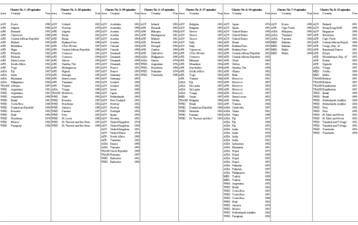
- 43 -
Table A2. Cluster Composition by Episode, Country, and Region
1339681v1-THE EFFECTIVENESS OF FISCAL PO.DOC November 21, 2001 (1:46 PM)
References
Alesina, Alberto, and Silvia Ardagna, 1998, “Tales of Fiscal Adjustment,” Economic Policy:
A European Forum, Vol. 27 (October), pp. 487-546.
Alesina, Alberto and Roberto Perotti, 1997, “Fiscal Adjustments in OECD Countries:
Composition and Macroeconomic Effects,” Staff Papers, International Monetary
Fund, Vol. 44, No. 2 (June), pp. 210-248.
Diday, E., and others, 1982, Elements d’analyse des donnees (Paris: Dunod).
Dunteman, G.H. 1980, Principal Components Analysis, in Series: Quantitative Applications
in the Social Sciences, 69 (London: Sage University Paper).
Everitt, B., 1974, Cluster Analysis (London: Heinemann).
Gavin, Michael, and Roberto Perotti, 1997, “Fiscal Policy in Latin America,” paper
presented at the Twelfth NBER Annual Macroeconomics Conference, April 5-4,
Cambridge MA.
Giavazzi, Francesco, Japelli, Tullio, and Marco Pagano, 2000, “Searching for Non-linear
Effectes of Fiscal Policy: Evidence from Industrila and Developing Countries,”
European Economic Review, Vol. 44, pp. 1259-89.
Giavazzi, Francesco and Marco Pagano, 1990, “Can Severe Fiscal Contractions be
Expansionary? Tales of Two Small European Countries,” NBER Macroeconomics
Annulas 5, pp. 111-6.
Giavazzi, Francesco and Marco Pagano, 1996, “Non-Keynesian Effects of Fiscal Policy
Changes: International Evidence and the Swedish Experience,” Swedish Economic
Policy Review, Vol. 3 (Spring), pp. 67-103.
Hemming, Richard, Michael Kell, and Selma Mahfouz, 2000, “The Effectiveness of Fiscal
Policy in Stimulating Economic Activity—A Review of the Literature,” SM/00/66,
IMF, March 2000.
IMF, 1998, World Economic Outlook, October 1998, pp.50-1.
Lane, Timothy, Atish Ghosh, Javier Hamann, Steven Phillips, Marianne Schultze-Ghattas,
and Tsidi Tsikata, 1999, “IMF-Supported Programs in Indonesia, Korea and
Thailand”, IMF Occasional Paper No. 178.
Lebart, L., A. Morineau, and M. Piron, 1995, Statistique Exploratoire Multidimensionelle,
(Paris: Dunod).
- -
45
Morrison, D.F., 1980, Multivariate Statistical Methods (Singapore: Mac Graw Hill
International Editions).
